A cell shows 05/06/2024 while the formula bar is the other day

05/06/2024 is not one day. On a United States spreadsheet the first number is the month, so the stored serial is May 6. A custom format can still paint 06/05/2024 in the cell. The formula bar follows the locale, not that paint. You read June 5 on the grid and May 6 in the bar, and no triangle appears.

This page is display versus the serial. It is not DATEVALUE day order, which parses a text date and can swap the same way. It is not dates stored as text. Keep the Google Sheets UI in English. Locale is File → Settings → Locale, not the display language.

Recreate it on a blank sheet

1. Open a blank spreadsheet. File → Settings. Set Display language to English. Set Locale to United States. Save. In A1 type typed.

What the locale stored. In A2 type 05/06/2024 and press Enter. Sheets accepts it. The formula bar shows a US date: month 5, day 6, so May 6, 2024. In B1 type iso. In B2 enter =TEXT(A2,"yyyy-mm-dd"). B2 is 2024-05-06. That ISO string is the day you actually have. There is no error.

Paint the other order on the same serial. Select A2. Format → Number → Custom date and time. Build a format that shows day, then month, then year (dd/mm/yyyy in the custom format box). Apply. A2 now displays 06/05/2024. The formula bar still shows the US reading, May 6. B2 is still 2024-05-06. You did not change the serial. You changed the paint. A reader who treats the cell as month/day now thinks it is June 5.

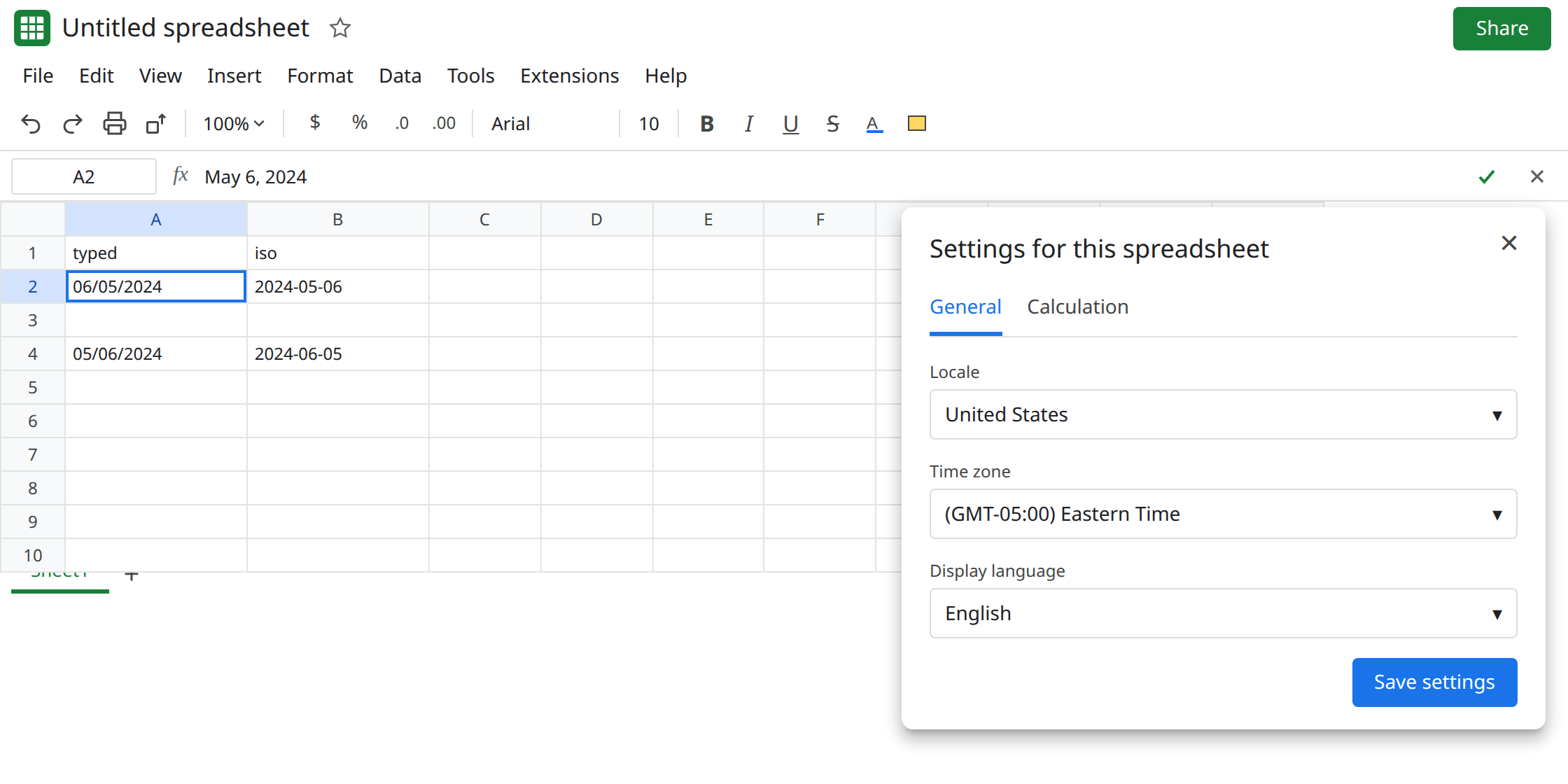
The June serial, for contrast. In A4 type 06/05/2024. On this US file that is June 5. =TEXT(A4,"yyyy-mm-dd") is 2024-06-05. Format A4 with the same day/month custom format and it displays 05/06/2024. A2 and A4 can be made to look like each other’s strings. The ISO column will not agree. Leave both formats in place.

Text is the other page. In A6 type an apostrophe, then 05/06/2024, so the cell stays text. ISTEXT(A6) is TRUE. DATEVALUE of that text follows the locale too, and it is DATEVALUE day order. A2 is not text. ISNUMBER(A2) is TRUE. A date serial is a number.

Split text to columns on a column of these strings can store the wrong day before you ever set a custom format. That walkthrough is split text to columns mangles dates.

What is actually wrong

• The value is decided when the date is entered, using File → Settings → Locale. United States reads 05/06/2024 as May 6. United Kingdom reads it as 5 June. The custom format runs later, on whatever serial is already stored.
• The formula bar shows the locale’s date, not the custom pattern. If the bar and the cell disagree about which number is the month, believe an ISO TEXT of the cell. B2 is that check.
• Formatting never re-parses the typed characters. Switching A2 to dd/mm/yyyy does not turn May 6 into June 5. Changing the locale afterward can reparse ambiguous input in some edits, and it will reparse DATEVALUE text. Do not flip locale to “fix” one column. It also changes argument separators. See locale parse error.
• NOW() jumping a calendar day is the time zone, not this format. See NOW / TODAY timezone.

This is not a date stored as text. Text is left-aligned, ISTEXT is TRUE, and XLOOKUP against a real date misses. See dates stored as text. A2 is a serial.

This is not DATEVALUE of 13/04/2024 on a US locale, which is #VALUE! because 13 is not a month. See DATEVALUE locale. Ambiguous 05/06 never errors. That is why it ships.

Fix

Leave A2 displaying the day/month pattern so the misleading paint stays on the sheet. Leave B2 as 2024-05-06.

Store the day with DATE, and display ISO when the order matters. In D1 type real. In D2 enter =DATE(2024,5,6). Format D2 as Format → Number → Date, or leave a neighbor =TEXT(D2,"yyyy-mm-dd") so the day is 2024-05-06 in a cell nobody can swap by eye. June 5 is =DATE(2024,6,5), not a different format of D2.

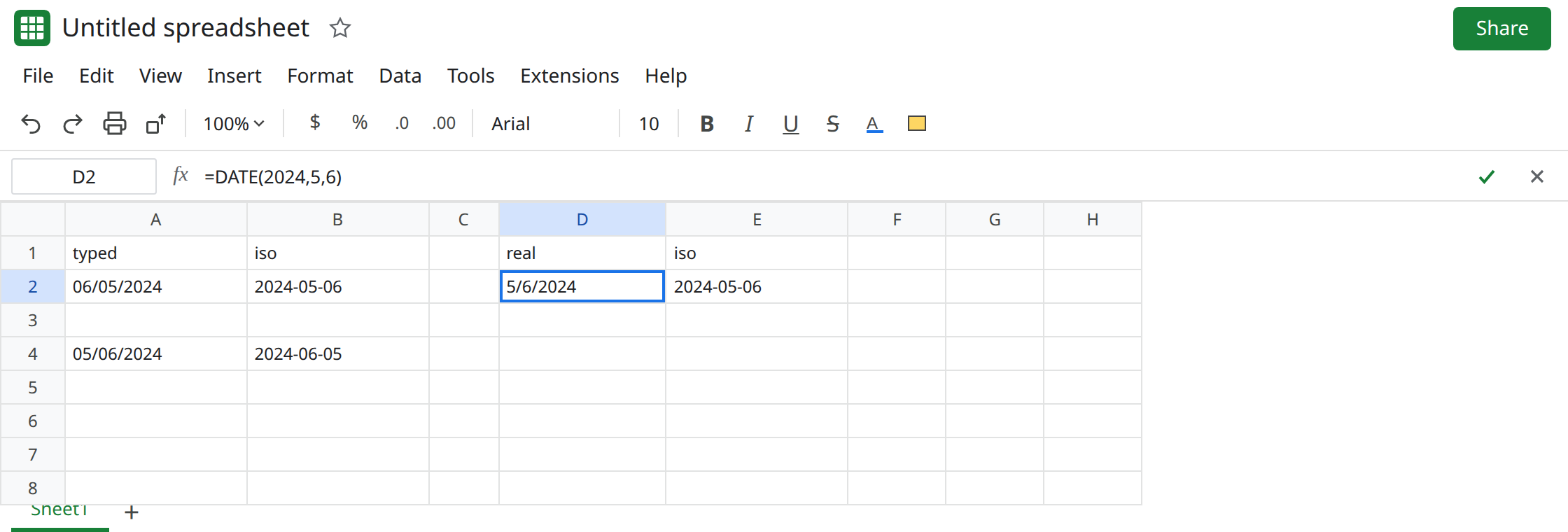
If the serial is already the wrong day, do not restyle it. Re-enter with DATE, or set the locale before typing ambiguous strings, then check TEXT(...,"yyyy-mm-dd") on the first row. A format that matches the locale (mm/dd/yyyy on United States) makes the cell and the formula bar tell the same story.

Do not wrap A2 in IFERROR. There is no error. The risk is a report dated a month off.

If the cell paint and the formula bar disagree, the format is not the serial. Read TEXT of the cell in yyyy-mm-dd. If the cell is text, you are on the DATEVALUE page, not this one.