Fix IRR and XIRR #NUM! in Google Sheets (same-sign cashflows, dates, guess)

IRR finds one rate for a list of cashflows. XIRR does the same with a date on each amount. #NUM! means the numbers are in domain for a spreadsheet, and these functions still cannot finish: every amount is positive (or every amount is negative), so there is no rate that crosses zero, or the optional guess never converges. A date column that is shorter than the amounts is a different failure (a size error). A date stored as text is #VALUE!.

This page is IRR / XIRR. It is not out of domain (SQRT of −1, LN(0), FACT(171)). It is not DATEVALUE locale. Keep the Google Sheets UI in English.

Recreate it on a blank sheet

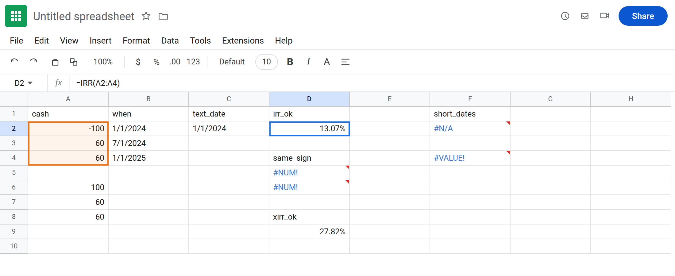
1. Open a blank spreadsheet. In A1 type cash. A2 -100. A3 60. A4 60. Money out, then two inflows. In B1 type when. In B2 enter =DATE(2024,1,1). B3 =DATE(2024,7,1). B4 =DATE(2025,1,1). Format B2:B4 as Date.

IRR that works. In D1 type irr_ok. In D2 enter =IRR(A2:A4). The cell shows a rate near 13% (about 0.13). Format D2 as a percent if it looks like 0.13. There is no error triangle. That cell is the control: one sign change, no guess argument (the default guess is 0.1).

Same sign. In A6 type 100. A7 60. A8 60. All inflows. In D4 type same_sign. In D5 enter =IRR(A6:A8). The cell shows #NUM!. There is no rate at which a string of only positive cashflows has net present value zero. Leave D5 broken. =XIRR(A6:A8,B2:B4) is #NUM! for the same reason. In D6 enter that XIRR. Leave D6 broken.

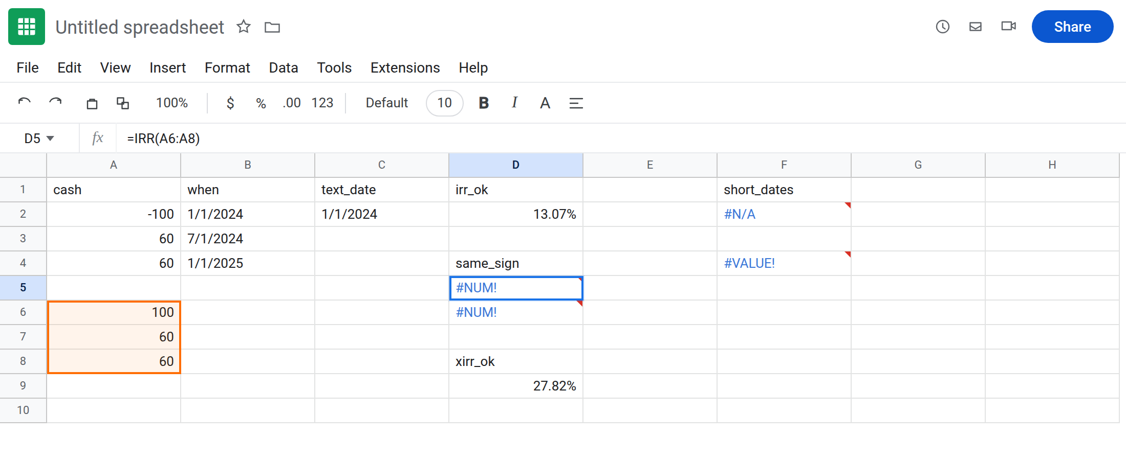
XIRR dates, aligned. In D8 type xirr_ok. In D9 enter =XIRR(A2:A4,B2:B4). A rate near the IRR result, not #NUM!. Dates line up with amounts: three and three. That row is the XIRR control.

Dates shorter than the cashflows. In F1 type short_dates. In F2 enter =XIRR(A2:A4,B2:B3). Four amounts? Three amounts and two dates. The cell shows #N/A or #VALUE!, not the same-sign #NUM!. The tooltip is about range size (XIRR’s two arrays differ). The signs in A2:A4 are already fine. Leave F2 broken.

A date stored as text. In C2 type '1/1/2024 (leading apostrophe, so the cell is text). C3 enter =DATE(2024,7,1). C4 enter =DATE(2025,1,1). =ISTEXT(C2) is TRUE. In F4 enter =XIRR(A2:A4,C2:C4). The signs and the row count are fine. The cell shows #VALUE! because C2 is not a date serial. See DATEVALUE locale if you meant to parse that string. Leave F4 as #VALUE!. Do not call it a bad guess.

Guess, only after a series already works. In D11 enter =IRR(A2:A4,0.1). It matches D2. The second argument is a decimal guess (0.1 means 10%), not a percent already multiplied into a whole number you still call “10 percent” without thinking. If a guess on this signed series returns #NUM! while D2 returns a rate, the guess did not converge. Leave D2 as the no-guess result. Do not demonstrate that by overwriting A2:A4.

Leave D5 and D6 as #NUM!. Leave F2 as the size error. Leave F4 as #VALUE!. Leave D2 and D9 as rates.

What is actually wrong

• IRR and XIRR need at least one negative amount and one positive amount. A project that only lists revenue (100, 60, 60) has no investment outflow. The functions return #NUM!. Flipping the sign of the first amount to negative is the usual fix when that amount really is money out. Do not flip a sign just to clear the triangle.
• Blank cells in the middle of the range are not a third sign. A blank is ignored or treated as zero depending on the call; a range that still has both signs can return a rate. A range you thought included -100 but started on row 6 does not. Look at the cells the formula names.
• XIRR pairs by position. Amount 1 with date 1. Two dates for three amounts cannot pair. That is F2, a size error. It is not “the rate does not exist.”
• The optional guess starts the search. The default is 10% (0.1). Passing 10 means a guess of 1000%. On a series that already solves with no guess, a wild guess can be #NUM! (did not converge). On a same-sign series, every guess is #NUM!. Change the cashflows, not the guess.
• XIRR dates must be real dates (ISNUMBER TRUE). Text that looks like 1/1/2024 is #VALUE!. Order can be unsorted; the first date is still the start of the schedule. A wrong rate with no triangle means the dates are paired with the wrong amounts (the range started one row too low), not that Sheets used SQRT.

This is not SQRT(-1). See out of domain. D5’s inputs are ordinary positives. The domain rule is about signs, not about a square root.

This is not #DIV/0!. See divide by zero. Nothing in D5 is a quotient.

This is not NPV showing a negative value. NPV returns a number. IRR returns a rate, or #NUM! when no rate works.

Fix

Leave D5, D6, and F2 broken.

Put an outflow in the list. Keep D2: =IRR(A2:A4) with -100, 60, 60. Keep D9: =XIRR(A2:A4,B2:B4) with three dates. If the first amount should be the investment, it is negative and the later amounts are the returns.

Match the date range to the amounts. B2:B4 with A2:A4, not B2:B3. If a date is text, replace it with =DATE(2024,1,1) or DATEVALUE of a string this locale accepts. Then call XIRR again.

Guess. Omit it until D2 works. If you must pass one, use a decimal near the rate you expect (0.1, not 10). If the no-guess formula works and the guessed one is #NUM!, delete the guess.

Do not wrap D5 in IFERROR and report a rate of 0. A same-sign list has no IRR. See IFERROR vs IFNA. IFNA does not catch #NUM!.

If IRR or XIRR is #NUM!, check for both signs before you touch the guess. If XIRR is #N/A or #VALUE! and the tooltip talks about size, count dates against amounts. If it is #VALUE! and a date cell is text, convert the date. SQRT is a different #NUM!.