

AVERAGEIF blank criteria: quotes, =, and an empty cell are not the same test
Updated
AVERAGEIF(criteria_range, criterion, [average_range]) treats three “blank” criteria as different tests. The criterion "" matches cells that are empty. The criterion "=" matches those same empty cells. A reference to a blank cell is not that test: Sheets coerces the blank criterion to 0, so you average rows whose criterion cell equals the number 0. Blank statuses drop out. A numeric zero status, if you have one, becomes the whole average. If you have no zero, the blank criterion is #DIV/0! because nothing numeric matched.
No numeric match at all, including a real category whose amounts are text, is AVERAGEIF #DIV/0!. A formula that returns "" versus a truly empty cell is ISBLANK vs empty. Keep the Google Sheets UI in English. Sheet Error is an independent formula-error library, not a Google product.
Recreate it on a blank sheet
Section titled “Recreate it on a blank sheet”- Open a blank spreadsheet. In A1 type
status, B1amt. A2Confirmed, B26. Leave A3 empty. B39. A4Pending, B410. A5Confirmed, B55. In A6 enter=""so the cell looks empty and is not. B620. A7 type0. B7100.
ISBLANK(A3) is TRUE. ISBLANK(A6) is FALSE. =A6="" is TRUE. The formula blank and the true blank both look empty. The 0 in A7 does not.
Quoted empty string. In D1 type quotes. In D2 enter =AVERAGEIF(A2:A7,"",B2:B7). D2 is 14.5. That is (9+20)/2. The true blank and the formula blank both match "". Confirmed, Pending, and the numeric 0 are out. The 100 is not in this average.
Equals sign in quotes. In D4 enter =AVERAGEIF(A2:A7,"=",B2:B7). D4 is 14.5. "=" is the “equals empty” operator. On this range it matches the same rows as "". It does not match A7. Leave D2 and D4 as 14.5.
Not-blank. In D6 enter =AVERAGEIF(A2:A7,"<>",B2:B7). D6 is (6+10+5+100)/4, which is 30.25. Both empty statuses are excluded. The numeric zero status is included, because 0 is not blank, and its amount 100 pulls the average up. A zero amount on a matched row would pull it the other way. Blanks in the amount column are skipped, not treated as zero. This criterion is the one people write when they mean “ignore blank status,” and it still counts a 0 status.
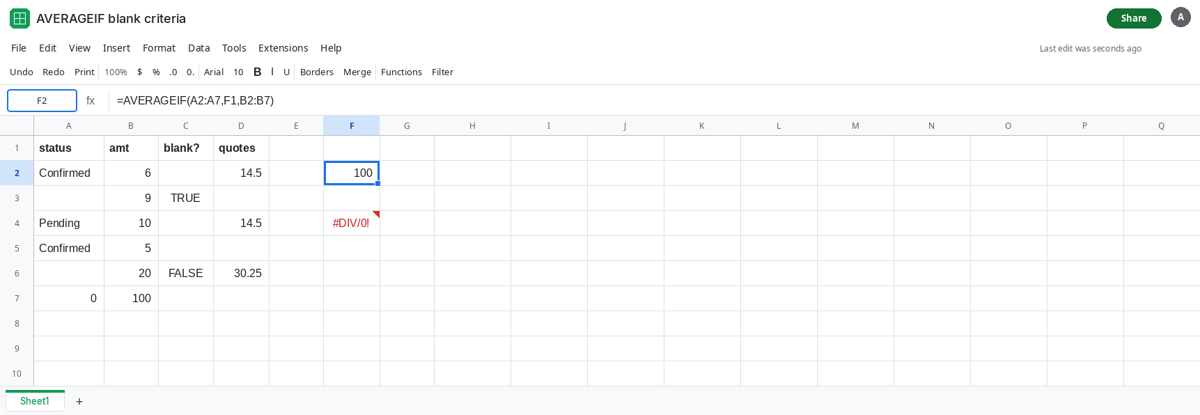
A blank cell as the criterion. Leave F1 empty. Do not type a space. In F2 enter =AVERAGEIF(A2:A7,F1,B2:B7). F2 is 100. F1 looks as empty as the criterion "", and the average is the zero-status row. The blank statuses and their 9 and 20 are not in it. Leave F2 as 100.
Delete the zero row’s match and the blank criterion breaks. In F4 enter =AVERAGEIF(A2:A6,F1,B2:B6). The range stops before A7. No status equals 0. F4 is #DIV/0!. That token is AVERAGEIF #DIV/0!. The cause here is the coerced zero criterion, not a misspelled category. Leave F4 broken.
Leave D2 as 14.5 and F2 as 100.
What is actually wrong
Section titled “What is actually wrong”""and"="are criteria that mean empty. They match a truly blank cell and a cell whose formula returns"". They do not match the number0.- A blank cell passed as the criterion is coerced to
0before the comparison.AVERAGEIFthen searches for status0. The average becomes that row’s amount, or#DIV/0!when no status is0. "<>"means not empty. It drops blank status and keeps a0status. It is not the opposite of a blank cell reference. The opposite of""is"<>". The blank cell reference is the zero test.- Amount blanks are skipped by
AVERAGEIFeven when the status matches. Amount zeros are included. Mixing those two is how an average moves without the status filter changing. See IF blank vs 0. ISBLANKis FALSE for A6. The criterion""still matches A6. If you only wanted truly empty cells,AVERAGEIF’s""is wider thanISBLANK. See ISBLANK vs empty.
This is not a range-size #VALUE!. See AVERAGEIFS range size when the tooltip says the ranges differ.
Leave F2 as 100 and D2 as 14.5. They are the two tests.
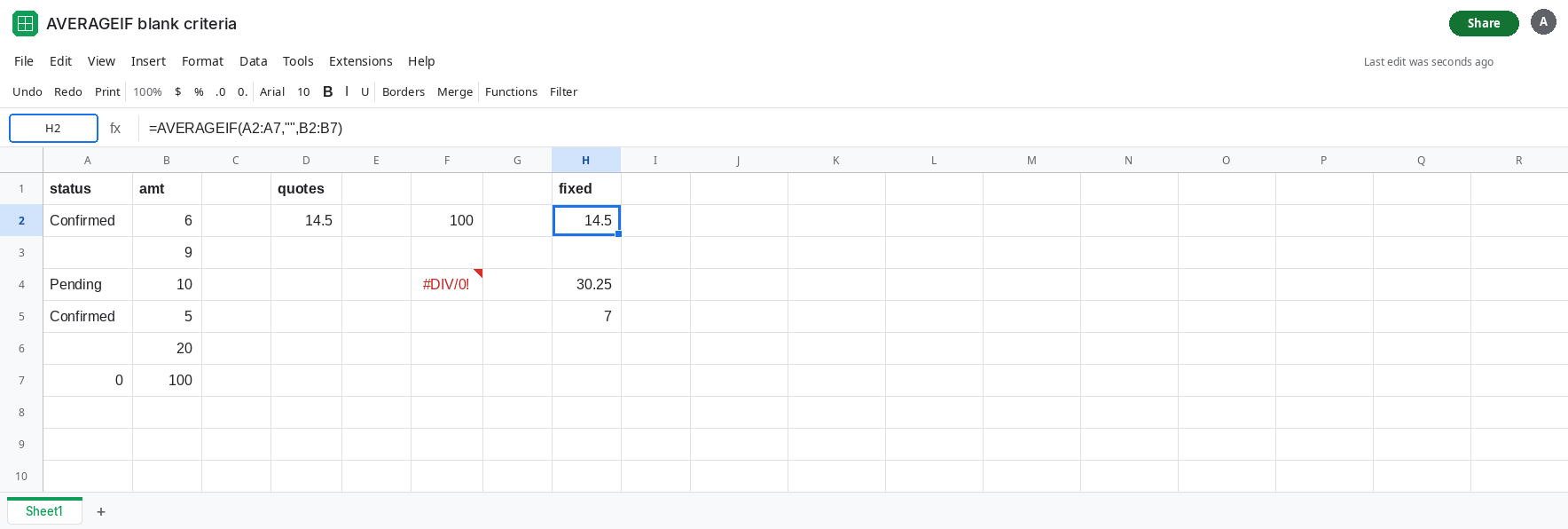
Average the blank statuses on purpose. In H2 enter =AVERAGEIF(A2:A7,"",B2:B7). H2 is 14.5. Type the quotes. Do not substitute a blank cell for them. "=" is the same match on this sheet if you prefer the operator form. Keep one of them.
Average everything except blank status, and decide about zero separately. In H4 enter =AVERAGEIF(A2:A7,"<>",B2:B7). H4 is 30.25, including the 100. To drop a zero status as well, in H5 enter =AVERAGEIFS(B2:B7,A2:A7,"<>",A2:A7,"<>0"). H5 is (6+10+5)/3, which is 7. AVERAGEIFS can hold both tests. A blank criterion cell cannot.
If the criterion has to come from a cell, do not leave that cell blank when you mean “match blanks.” In F1 type ="" (a formula that returns empty) or use =IF(F1="",AVERAGEIF(A2:A7,"",B2:B7),AVERAGEIF(A2:A7,F1,B2:B7)) so an unused picker means the blank-status average, and a typed 0 still means zero. Read F1’s formula bar before you trust F2.
If the criterion argument is a blank cell and the average equals the row where the status is 0, you are matching zero. If the criterion is "" and the average includes formula blanks, that is the empty-string match. If the cell is #DIV/0!, no numeric amount matched the criterion you actually passed. See AVERAGEIF #DIV/0!.