Fix AVERAGEIF #DIV/0! in Google Sheets (no numeric match)

AVERAGEIF(range, criterion, [average_range]) averages the cells that match. Internally that is a sum divided by a count of numeric matches. When that count is zero, Sheets returns #DIV/0!. The criterion can miss every row, or it can hit rows whose average cells are blank or text (TBD). That is not =A2/B2 with a zero typed in the divisor.

This page is AVERAGEIF empty-average. It is not divide by zero (10/0, blank divisor). It is not COUNTIFS range size. It is not [AVERAGE of a whole range with no numbers] as a different layout — the function here is AVERAGEIF. Keep the Google Sheets UI in English.

Recreate it on a blank sheet

1. Open a blank spreadsheet. In A1 type region, B1 score. A2 East. B2 10. A3 East. B3 8. A4 West. B4 TBD as text. A5 West. Leave B5 empty. West has no numeric scores. East has two.

AVERAGEIF West. In D1 type west. In D2 enter =AVERAGEIF(A2:A5,"West",B2:B5). The cell shows #DIV/0!. Tooltip: Function DIVIDE parameter 2 cannot be zero (or AVERAGEIF of no numeric values). West matched two rows. Neither is a number. Leave D2 broken.

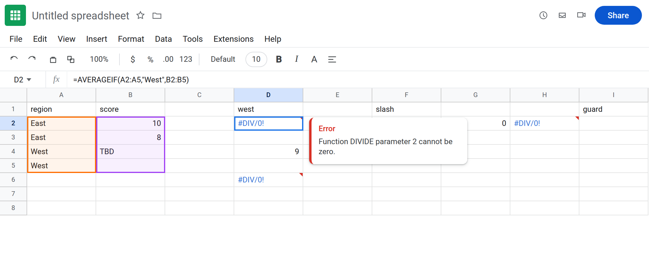
AVERAGEIF East (control). In D4 enter =AVERAGEIF(A2:A5,"East",B2:B5). The cell shows 9. Same function, numeric matches.

Criterion that hits nobody. In D6 enter =AVERAGEIF(A2:A5,"North",B2:B5). #DIV/0! again. No North rows. Leave D6 broken.

Slash contrast. In F1 type slash. F2 10. G2 0. In H2 enter =F2/G2. #DIV/0!. That primer is divide by zero. Leave H2 as contrast. Do not “fix” D2 by changing G2.

AVERAGE of blanks. In D8 enter =AVERAGE(B4:B5). Also #DIV/0! (no numeric values in the range). Sibling, no criterion. Leave D8 if it errors. The recreate you came here for is D2.

Leave D2 and D6 broken. Leave D4 as 9.

What is actually wrong

• AVERAGEIF divides by how many numbers matched, not how many rows matched. Two West rows with TBD and blank still count as zero numbers.
• A criterion miss (North) is the same #DIV/0!. There is no #N/A for “no match” on this function. That token is FILTER / XLOOKUP territory.
• TBD is text. It does not coerce to 0 inside AVERAGEIF. A 0 would be a numeric match and would pull the average down. Blank is skipped, not a zero, for AVERAGE.
• Range size still matters: AVERAGEIF(A2:A5,"West",B2:B6) can #VALUE! on some builds if the average range length differs. That is the COUNTIFS-style size bug, not this #DIV/0!. See COUNTIFS range size and MAXIFS range size.

This is not QUERY avg(B) on mixed types (#VALUE! AVG_SUM). See QUERY group by. D2 ran. The count was zero.

This is not #N/A. See what #N/A means.

Fix

Leave D2, D6, and H2 broken.

When West should have scores, type numbers in B4 and B5. D2 becomes a number. Put TBD back if you want the error visible next to the fix cell.

When zero matches should print blank: In I2 enter =IF(COUNTIF(A2:A5,"West")=0,"",IF(COUNTIFS(A2:A5,"West",B2:B5,">=0")+COUNTIFS(A2:A5,"West",B2:B5,"<0")=0,"",AVERAGEIF(A2:A5,"West",B2:B5))) is heavy. Simpler: =IFERROR(AVERAGEIF(A2:A5,"West",B2:B5),"") only if every error on that cell should vanish. Prefer counting numbers: =IF(COUNT(FILTER(B2:B5,A2:A5="West"))=0,"",AVERAGEIF(A2:A5,"West",B2:B5)).

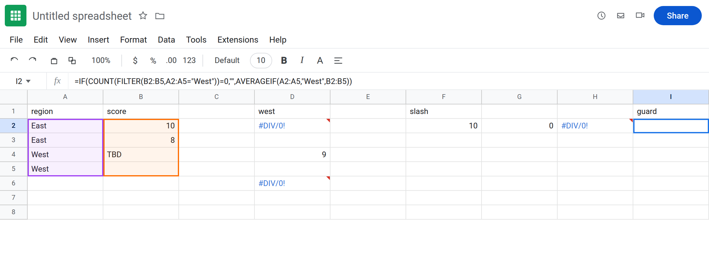
Keep D4 as proof East works. See IFERROR vs IFNA. IFNA will not catch #DIV/0!.

If #DIV/0! and the formula is AVERAGEIF, count numeric matches. If the formula is A2/B2, the other primer. If #VALUE!, check range lengths.

No numeric match vs slash vs AVERAGE of empty

AVERAGEIF West with TBD/blank → #DIV/0! (D2). This page.

=10/0 → #DIV/0! (divide by zero). Typed divisor.

AVERAGE of a range with no numbers → same token, no criterion. Guard with COUNT of that range. Do not import a slash IF(B2=0,"",…) onto D2 until you have looked at COUNT(FILTER(...)).