Legacy Excel CSE arrays become values, a parse error, or #NAME? in Google Sheets

Older Excel used Ctrl+Shift+Enter to enter an array formula. Excel stored it with braces, {=SUM(A2:A4*B2:B4)}, and calculated the whole array. Google Sheets does not have that keystroke. Pressing Ctrl+Shift+Enter in Sheets edits the cell. It does not create a CSE array and it does not add braces. When the .xlsx opens in Sheets, look at the formula bar. An empty bar means the block is values. A bar that still starts with {= is not a Sheets array. A bar that contains _xlfn. is #NAME?. The numbers on the grid can look finished either way.

Excel’s newer dynamic spills, and the A1# spill reference, are Excel spill to values. A Sheets formula that cannot spill because a cell is in the way is array result was not expanded. Keep the Google Sheets UI in English. Sheet Error is not Microsoft and not Google.

Recreate it on a blank sheet

1. You need Excel for the first half and Google Sheets for the second. In Excel, in A1 type qty, B1 price. A2 2, B2 5. A3 3, B3 4. A4 1, B4 10. The sum of the products is 2*5+3*4+1*10, which is 32.

A legacy array formula in Excel. In D2 enter =SUM(A2:A4*B2:B4) and confirm it with Ctrl+Shift+Enter if your Excel still requires that for an array. The formula bar shows braces, {=SUM(A2:A4*B2:B4)}, on those older builds. D2 shows 32. A current Excel may accept the formula without braces and spill or return 32 as a dynamic array. If your Excel never shows braces, this file is not the legacy case. Use a workbook that still has {=...} in the bar, or type the lesson from the Sheets side below. The control in Excel is a live formula that equals 32.

Open it in Sheets. Save as .xlsx. In Google Sheets, File → Import → Upload and open the file. Click D2, or whichever cell shows 32.

Read the formula bar. You are looking for one of these:

• The bar is empty and D2 is the value 32. Change A2 from 2 to 9. D2 stays 32. The array was flattened to a value. Leave it flattened.
• The bar shows {=SUM(A2:A4*B2:B4)} or another leading {=. The cell is #ERROR! with Formula parse error, or it does not calculate as an array. { in Sheets starts an array literal, not an Excel CSE formula. Leave it broken.
• The bar shows a name with _xlfn. in front of a function. The cell is #NAME?. That prefix is Excel’s. Sheets does not have a function by that name. Leave it as #NAME?. See unknown function.

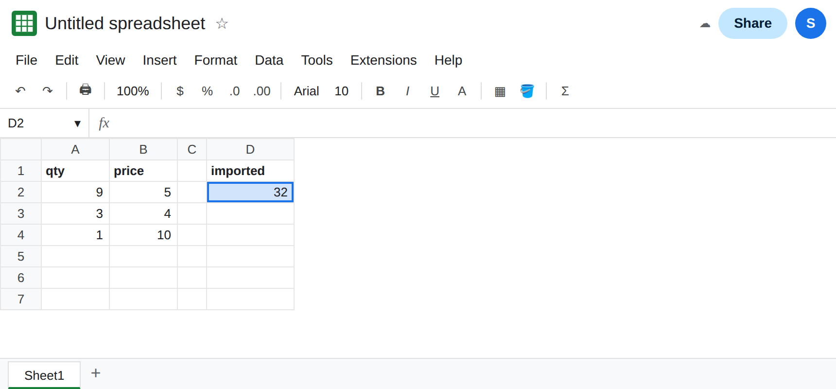
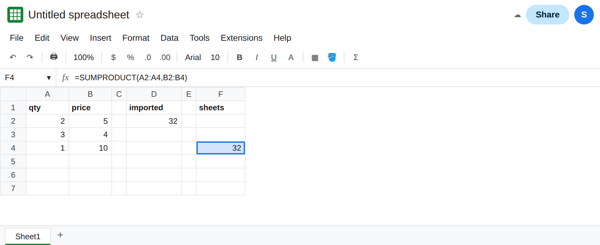
Sheets will not add the braces for you. On a blank area of the Sheets file, in F2, type =SUM(A2:A4*B2:B4) and press Ctrl+Shift+Enter. The bar does not gain { }. You either get a parse result, a single value, or #VALUE!, depending on the build. You do not get an Excel CSE array. In F4 enter =SUMPRODUCT(A2:A4,B2:B4). F4 shows 32, and it follows A2 when you change A2. That cell is the Sheets control. Leave the imported D2 in the broken or static state.

This is not Excel spill to values. That page is UNIQUE, FILTER, and A1#. CSE braces are older. A file can contain both. The bar tells you which one you imported.

What is actually wrong

• CSE was a way to ask Excel to evaluate a formula as an array. Sheets uses ARRAYFORMULA, or functions that already accept arrays, such as SUMPRODUCT. The braces are not a wrapper Sheets keeps.
• An empty formula bar is values. Editing A2 will not change D2. The import kept the last calculated number. See the same test on Excel spill to values.
• {=SUM(...)} is not “the same formula with a reminder that it is an array.” The { is syntax. Sheets tries to parse an array constant and fails, or parses something you did not mean.
• _xlfn. marks a function Excel stored under an internal name. #NAME? means that name is not a Sheets function. Removing the prefix only helps when the rest of the name exists in Sheets. Guessing is how you trade #NAME? for #ERROR!.
• =SUM(A2:A4*B2:B4) without a wrapper is not a reliable port. SUMPRODUCT is the product-sum. ARRAYFORMULA is the wrapper when you need one. Dragging a formula down is a different #REF!. See ARRAYFORMULA drag.
• Locale separators still apply to whatever you retype. A comma formula on a semicolon locale is locale parse error. That parse error is not the CSE braces. Read the bar before you change locale.

Fix

Leave the imported cell as values or as {=...} so the failed port stays visible.

Retype the calculation in Sheets. Keep F4: =SUMPRODUCT(A2:A4,B2:B4). It shows 32 and it changes when A2 changes. The array form, when you want it, is =ARRAYFORMULA(SUM(A2:A4*B2:B4)). Do not type braces around either formula.

For a single-column condition, prefer the function that already takes a range. SUMIF or SUMIFS replaces a CSE SUM(IF(...)). You do not press Ctrl+Shift+Enter after it.

A #NAME? with _xlfn. needs a Sheets function of the same job. Delete the prefix only when you recognize the name. Otherwise rewrite the cell. See unknown function.

Do not paste the braced formula into IFERROR. You would hide a parse error and keep a blank where 32 should recalculate. See IFERROR vs IFNA.

If the formula bar is empty, the import stored values. Retype SUMPRODUCT or ARRAYFORMULA. If the bar starts with {=, delete the braces and use a Sheets array. If the bar contains _xlfn., you are on #NAME?. If the bar shows A1#, you are on the dynamic-spill page, not this one.