T() returns a blank when the cell is a number

T(value) returns text, and only text. If the value is already text, you get that text. If the value is a number, a date serial, or a boolean, T returns an empty string. The cell looks blank. LEN of the result is 0. A numeric id such as 1042 disappears. Whatever you concatenate or look up next is working with a blank key, and the formula does not show #VALUE! for the conversion itself.

N does the opposite conversion and turns text into 0. That page is N() text to 0. A blank that was really empty, versus a formula that returned "", is ISBLANK vs empty. Keep the Google Sheets UI in English. Sheet Error is an independent formula-error library, not a Google product.

Recreate it on a blank sheet

1. Open a blank spreadsheet. In A1 type id. A2 type 1042 as a number. A3 type 1043 as a number. A4 type West as text. Two numeric ids and one text code. You want all three kept as text keys.

T keeps the word and drops the numbers. In C1 type t. In C2 enter =T(A2). C2 looks blank. In C3 enter =T(A3). C3 looks blank. In C4 enter =T(A4). C4 is West. In D2 enter =LEN(C2). D2 is 0. In D4 enter =LEN(C4). D4 is 4. =C2="" is TRUE. The id is gone. There is no error triangle on C2.

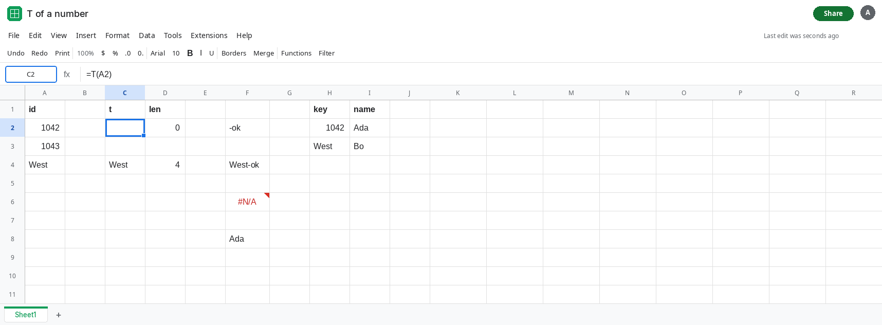
A join inherits the blank. In F2 enter =T(A2)&"-ok". F2 is -ok. The id never reached the dash. In F4 enter =T(A4)&"-ok". F4 is West-ok. Same formula. Only the text code survived.

A lookup for the blank. In H1 type key, I1 name. H2 type 1042. I2 type Ada. H3 type West. I3 type Bo. In F6 enter =VLOOKUP(C2,H2:I3,2,FALSE). The search key is C2, which is T of the number. F6 is #N/A. The id 1042 is sitting in H2. The key you searched was blank. Leave F6 as #N/A.

The number was fine before T. In F8 enter =VLOOKUP(A2,H2:I3,2,FALSE). F8 is Ada. The lookup works when the key is the original number. T was the step that removed it.

Leave C2 blank, F2 as -ok, and F6 as #N/A.

What is actually wrong

• T is a filter, not a formatter. It answers “if this is text, hand it back; otherwise hand back empty.” A numeric id is not text, even when it looks like a code on the sheet.
• The empty result is a zero-length string, not a cleared cell and not #VALUE!. LEN is 0. ISBLANK on C2 is FALSE, because a formula returned "". See ISBLANK vs empty.
• Downstream functions trust that string. Concatenation glues the dash to nothing. VLOOKUP searches for blank and returns #N/A even though the numeric id exists in the table.
• ARRAYFORMULA(T(A2:A4)) does this to every row. The text code remains. The ids become a blank spill. The spill is not a blocked array. See SORT / UNIQUE spill only if the next cell is already filled and the error is #REF!.
• TO_TEXT and TEXT format a number as text. T refuses the number. They are not substitutes for each other.

This is not wrong type from adding text to a number. T succeeded. The damage is the blank.

Fix

Leave C2, F2, and F6 as the broken chain.

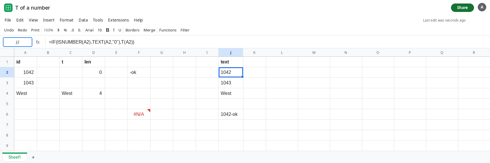
Turn the id into text on purpose. In J2 enter =IF(ISNUMBER(A2),TEXT(A2,"0"),T(A2)). Fill J2:J4. J2 is 1042, J3 is 1043, J4 is West. All three are text. ISTEXT(J2) is TRUE. In J6 enter =J2&"-ok". J6 is 1042-ok.

Or skip T when the column is an id. =TEXT(A2,"0") on a numeric id is 1042. On the word West it returns West as well in Sheets, because TEXT of text that does not match a number format often comes back unchanged. If a code must keep leading zeros, store it as text from the import and do not run it through T or through a 0 format. See CSV text vs number.

Look up the original cell. Point VLOOKUP at A2, not at T(A2), when A2 is the id you imported. F8 already returns Ada.

If T of a cell is blank and the formula bar of the source shows digits with no leading apostrophe, the source is a number and T dropped it. If the source formula bar shows an apostrophe, the value is already text and T should keep it. If the lookup key is blank and #N/A, the key was erased before the search.