Fix XMATCH #N/A in Google Sheets

XMATCH returns the relative position of a key in a range. #N/A means it did not find a position it is allowed to return. That can be a real miss (default exact match, key absent). It can also be a binary search_mode (2 or -2) on a range that is not sorted the way that mode requires. Both cells show #N/A. They are not the same problem.

This page is XMATCH. It is not MATCH #N/A (MATCH defaults to approximate 1; you pass 0 for skus). It is not XLOOKUP #N/A (XLOOKUP returns a value from another range, plus if_not_found). It is not what #N/A means as a general primer, though that page is the right start if you only know the error value.

Recreate it on a blank sheet

1. Open a blank spreadsheet. In A1 type bay. In A2 type BAY-12. A3 BAY-40. A4 BAY-28. The list is not sorted. D1 lookup. D2 BAY-99. D3 BAY-28.

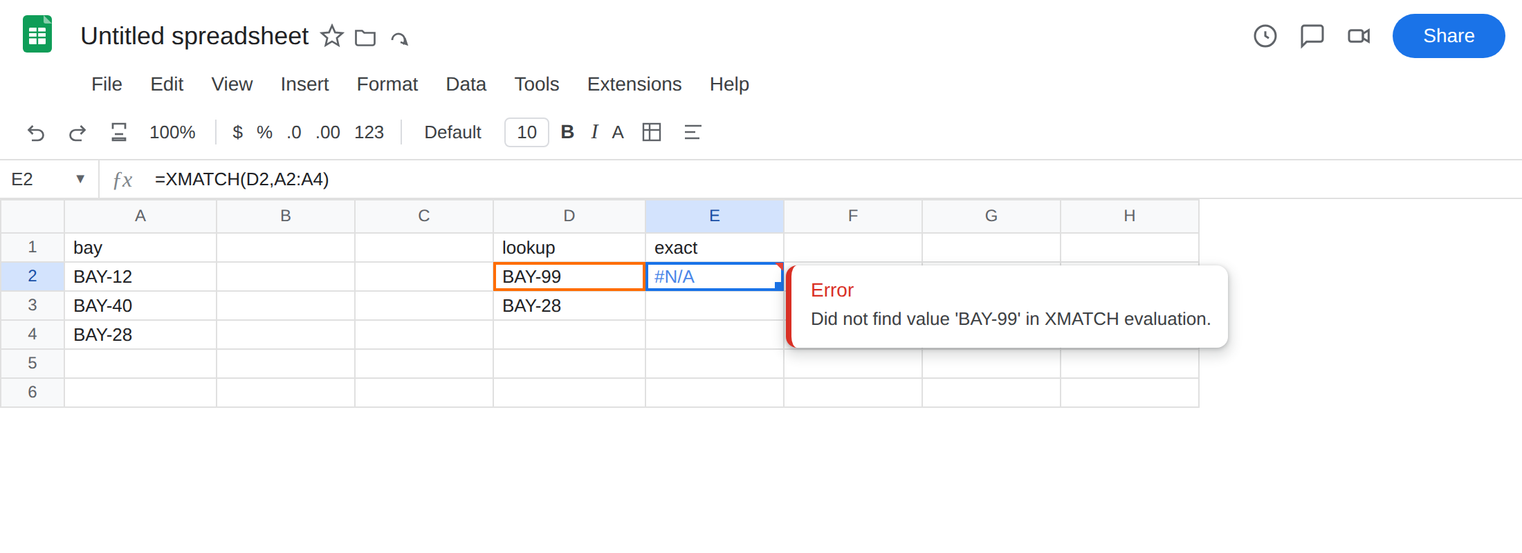
Exact miss. In E1 type exact. In E2 enter =XMATCH(D2,A2:A4). The cell shows #N/A. The tooltip is Did not find value ‘BAY-99’ in XMATCH evaluation. Default match_mode is exact (0). BAY-99 is not in A2:A4. Leave E2 broken.

Exact hit on the unsorted list. In E3 enter =XMATCH(D3,A2:A4). The cell shows 3. Bay BAY-28 is the third cell in A2:A4. Default exact match does not care about sort order.

Binary search_mode on the same unsorted list. In F1 type binary. In F2 enter =XMATCH(D3,A2:A4,0,2). Fourth argument 2 is binary search, first-to-last, range must be sorted ascending. A2:A4 is BAY-12, BAY-40, BAY-28. F2 is #N/A or a wrong position — not 3. Leave F2 if it is not 3.

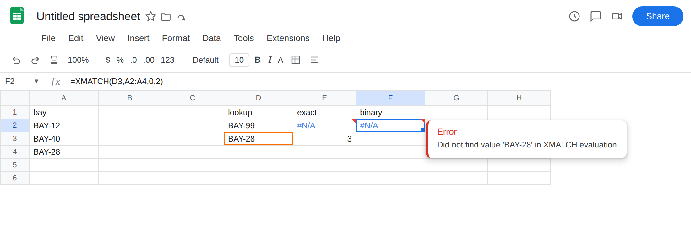
Confirm the exact miss. Type BAY-28 in D2. E2 becomes 3. Put BAY-99 back so #N/A returns. F2 will not toggle the same way: BAY-28 is on the sheet and binary search can still fail. -2 (binary descending) on this unsorted list is the same class of failure as F2.

What is actually wrong

• XMATCH(key, range) with no extra arguments is exact. #N/A means the key is not in the range (or it does not actually match: number vs text, a trailing space). D2 BAY-99 is the clean miss.
• The fourth argument is search_mode, not match type. 1 (default) walks first to last. -1 walks last to first (last match). 2 and -2 are binary. Binary needs a sorted range. BAY-12, BAY-40, BAY-28 is not sorted. Binary #N/A is not “BAY-28 is missing.”
• The third argument is match_mode: 0 exact (default), -1 exact or next smaller, 1 exact or next larger, 2 wildcard. Wildcard 2 is not binary search. Do not mix those 2s. XMATCH(D3,A2:A4,2) is wildcard match_mode. XMATCH(D3,A2:A4,0,2) is exact plus binary search_mode.
• The result is a position, not a name. 3 means the third cell of A2:A4. People wrap INDEX around it to pull another column. The #N/A still comes from XMATCH. Fix XMATCH first. This is not MATCH. MATCH’s third argument is match_type, and omitting it is approximate 1. XMATCH omitting extras is exact. See MATCH #N/A. Do not “fix” XMATCH by passing 0 the way you fix MATCH — it already defaulted to exact.

This is not XLOOKUP returning a value. XLOOKUP has if_not_found. XMATCH does not. See XLOOKUP #N/A.

This is not FILTER with zero rows. See FILTER no match.

Fix

Leave E2 as the exact miss. Leave F2 as the binary failure.

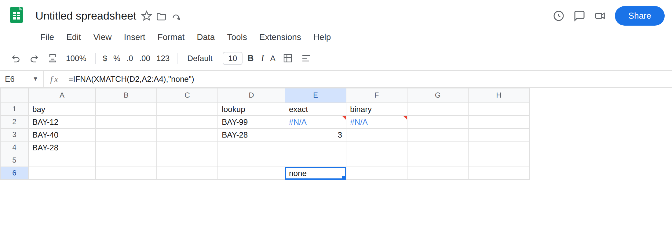
Bay lookups: leave search_mode off, or pass 1. Keep E3: =XMATCH(D3,A2:A4) returns 3. For a miss that may print a label, in E6 enter =IFNA(XMATCH(D2,A2:A4),"none"). The cell shows none. Use IFNA, not IFERROR. See IFERROR vs IFNA. Do not wrap F2. Binary #N/A on an unsorted list is a search_mode bug, not a missing bay.

If you actually want binary search. Sort ascending for 2 (or descending for -2), then pass that mode on a long sorted id list. Short bay lists use the default walk. Last match in a repeating column is search_mode -1 (reverse linear), not -2.

If XMATCH is #N/A and you can see the key, read the fourth argument. Default plus a visible key is type or spaces. 2 or -2 on an unsorted column is this page.

XMATCH search_mode vs MATCH match_type

MATCH packs “exact vs approximate” into one number: 0, 1, -1. Approximate 1 / -1 requires sorted data. People omit the argument and get approximate by accident. That story lives on MATCH #N/A.

XMATCH splits the idea. Exact is the default match_mode. Walking the list is the default search_mode. Binary is opt-in (2 / -2). If you migrated MATCH(...,0) to XMATCH and then copied a 2 from a blog that meant “wildcard” or “binary,” you can recreate this miss on a key that is sitting in the column.

Need the name in the next column, not the position? That is XLOOKUP, not a bigger XMATCH. =XLOOKUP(D3,A2:A4,B2:B4) if B holds names. Stay on XMATCH when the thing you want is 3.