Fix MMULT #VALUE! in Google Sheets (inner dimensions)

MMULT(matrix1, matrix2) multiplies two matrices. If matrix1 is m × n, matrix2 must be n × p. The product is m × p. #VALUE! here means those inner sizes (n) do not match — 2×3 next to 2×2 has inner 3 vs 2. The numbers can be fine. The shapes are not. Text in a matrix is a different #VALUE! (wrong type inside).

This page is MMULT inner dimensions. It is not wrong type (10 + pcs) as the generic primer. It is not FILTER range size. It is not COUNTIFS range size. Keep the Google Sheets UI in English.

Recreate it on a blank sheet

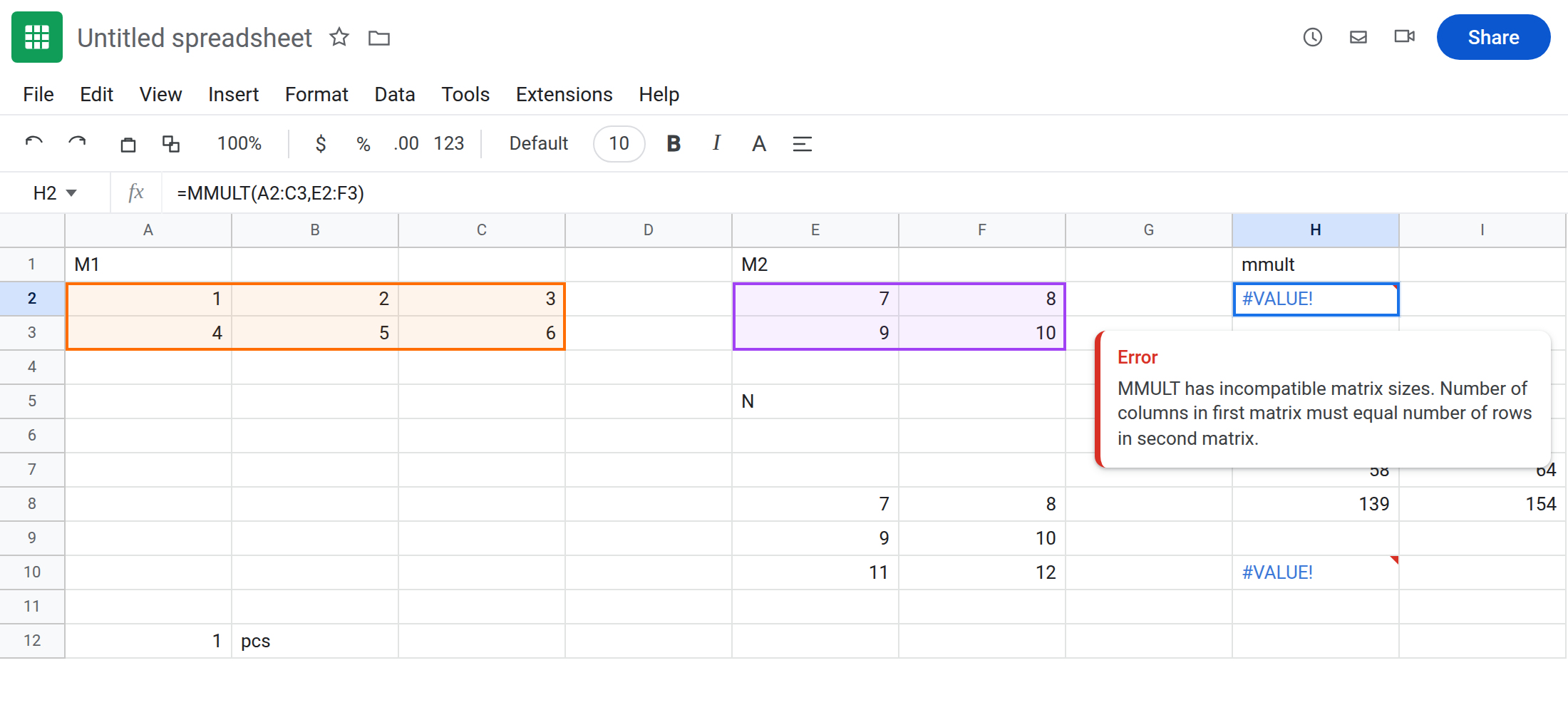
1. Open a blank spreadsheet. In A1 type M1. A2 1. B2 2. C2 3. A3 4. B3 5. C3 6. That block is 2×3. In E1 type M2. E2 7. F2 8. E3 9. F3 10. That block is 2×2.

Inner 3 vs 2. In H1 type mmult. In H2 enter =MMULT(A2:C3,E2:F3). The cell shows #VALUE!. Tooltip: MMULT has incompatible matrix sizes (or Function MMULT parameter 2 does not have the right row count). 3 columns cannot meet 2 rows. Leave H2 broken.

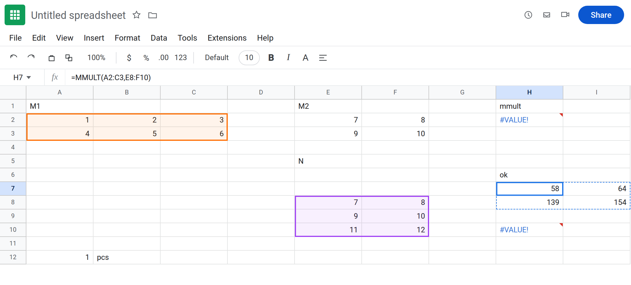
A product that fits. In E6 type N. E6 stay as label in E5 if needed. Put a 3×2 in E8:F10: E8 7. F8 8. E9 9. F9 10. E10 11. F10 12. In H6 type ok. Leave H7:I8 empty. In H7 enter =MMULT(A2:C3,E8:F10). 2×3 times 3×2 = 2×2 spill (58 / 64 / 139 / 154 if you multiply by hand: row1·col1 = 1·7+2·9+3·11 = 58). That block is the control.

TRANSPOSE to force a fit (when you meant that). In H10 enter =MMULT(A2:C3,TRANSPOSE(E2:F3)). TRANSPOSE of 2×2 is still 2×2 — still #VALUE! against 2×3. Leave H10 broken. TRANSPOSE of a 2×3 is 3×2, which would fit: in H12 enter =MMULT(A2:C3,TRANSPOSE(A2:C3)) only if you wanted Gram-style square products — optional control, 2×2.

Text inside a legal shape. In A12 1. B12 pcs. A13 2. B13 3. Two-by-two with pcs. In E12 1. F12 0. E13 0. F13 1. In H14 enter =MMULT(A12:B13,E12:F13). #VALUE! from type, not from 2 vs 2. Leave H14 broken as contrast. See wrong type.

Leave H2 as the size error. Leave H7 as the working spill. Leave H14 as text.

What is actually wrong

• Inner dimensions are the shared n: columns of the first, rows of the second. Count them. 3 ≠ 2 is H2.
• MMULT spills m×p. Occupied cells in that rectangle are #REF!, a different token. See SORT / UNIQUE spill for overwrite in general. If H7 were #REF!, clear I7.
• TRANSPOSE swaps rows and columns. It only fixes MMULT if that swap is the n you needed. Transposing a square does not create a 3.
• One text cell in an otherwise legal pair is #VALUE! without a size tooltip. H14. Read the tooltip before you add a row.

This is not FILTER Expected row count. See FILTER range size.

This is not MAXIFS different size. See MAXIFS / MINIFS size.

This is not MAP different size. See BYROW / MAP LAMBDA.

Fix

Leave H2, H10, and H14 broken.

Match n. Keep H7: =MMULT(A2:C3,E8:F10) with the 3×2 in E8:F10. Or shrink the first matrix to 2×2 (A2:B3) if the third column should not participate: =MMULT(A2:B3,E2:F3) also works (2×2 times 2×2).

Do not wrap H2 in IFERROR so a shape bug prints 0. See IFERROR vs IFNA. IFNA will not catch #VALUE!.

If #VALUE! and the tooltip names matrix sizes, count n. If it names text / coercion, find pcs. If #REF!, clear the spill. If you needed element-wise multiply, that is A2:B3*E2:F3 (same shape), not MMULT.

Inner n vs element-wise vs MAP size

MMULT 2×3 · 2×2 → #VALUE! (H2). Shared n missing.

A2:B3*E2:F3 → element-wise, same dimensions required, not a matrix product.

MAP two arrays of different length → BYROW / MAP LAMBDA. Different function, “different size” in the tooltip. Read MMULT in the formula bar before you equalize FILTER-style row counts.