NPV treats the first cashflow as end of period 1, not time zero

NPV(rate, value1, value2, ...) discounts value1 by one full period. That argument is the cashflow at the end of period 1, not the cashflow today. An opening outlay placed inside the function is discounted as if it happened one period later. The cell shows a number. There is no #NUM!, no #VALUE!, and no triangle. A second formula that adds the outlay outside NPV shows a different number on the same cashflows.

This is not a recommendation to invest, borrow, or accept a project. The figures below only show timing. Sign errors and a rate that never converges are IRR / XIRR #NUM!. IRR is a different function. Do not “fix” a timing gap by switching to IRR and reading the rate as a value.

Recreate it on a blank sheet

1. Open a blank spreadsheet. Locale United States, Google Sheets UI in English. In A1 type t, B1 cf. A2 0, B2 -1000. A3 1, B3 400. A4 2, B4 400. A5 3, B5 400. The -1000 is time zero. The three 400s are the ends of the next three periods. In D1 type rate. D2 0.1.

Outlay outside, which matches the labels in column A. In F1 type time0_outside. In F2 enter =B2+NPV(D2,B3:B5). Format F2 as a number with two decimal places. The cell shows -5.26. NPV discounts only 400, 400, 400. B2 is added at full value because it is already at time zero.

Outlay inside. In F4 type all_inside. In F5 enter =NPV(D2,B2:B5). Format F5 with two decimal places. The cell shows -4.78. The -1000 was discounted one period, then the three receipts were discounted as periods 2, 3, and 4. No error triangle. The two cells do not match.

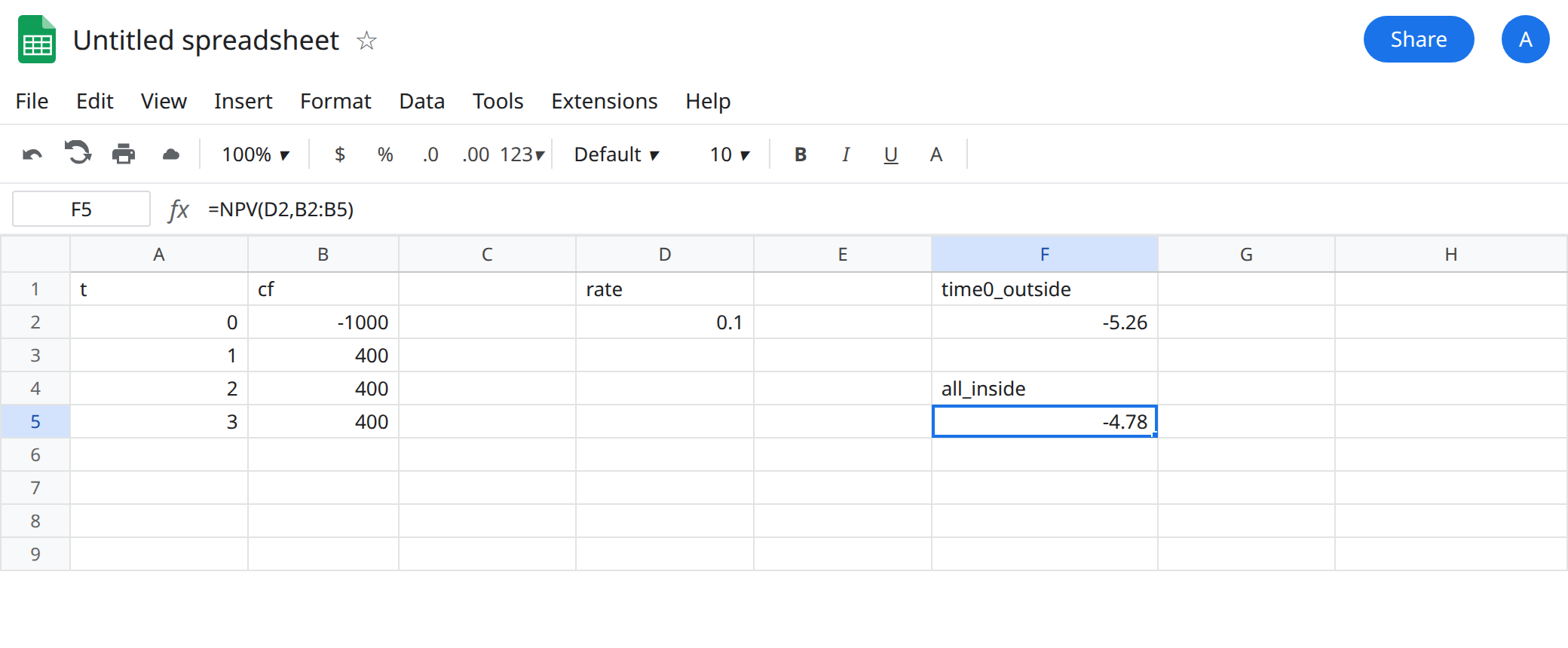
Why those two displays. At 10 percent, the three receipts discounted one, two, and three periods sum to about 994.74. Plus -1000 is about -5.26 (F2). Put -1000 inside and it is divided by 1.1 first (about -909.09), and each receipt moves one period further out. The total is about -4.78 (F5). Your sheet may show more decimals before you format. The formatted pair -5.26 and -4.78 is the check. If F2 and F5 match, the range in one of them is wrong.

Leave F5 as the shifted timing. Do not overwrite it with F2’s formula. You want both numbers on the sheet.

What is actually wrong

• Google Sheets, like the usual spreadsheet definition, takes the first NPV cashflow as end of period 1. There is no argument for “this list starts at time zero.” F5 is not a broken rate. D2 is a fine 0.1. The range is one cell too far to the left.
• The shift hits every later cashflow, not only the outlay. Inside F5, the first 400 is treated as period 2. A project that looked slightly negative can change magnitude, and a different set of cashflows can change sign. This example stays negative either way (-5.26 versus -4.78) so you can see a pure timing gap without a sign story. Do not generalize “-4.78 means accept.” Neither display is advice.
• Blank cells inside the range are part of the series. A blank between receipts is a zero cashflow for that period, which inserts a period. That is another timing bug, and it is also silent. Do not leave a note in B4 and point NPV through it.
• Text in the range is ignored by NPV the way SUM ignores text, or it can throw #VALUE! depending on the values. A short series with no triangle is the SUMIF text-number problem applied to cash. F5’s problem is not text. ISNUMBER on B2:B5 is TRUE.
• IRR(B2:B5) solves a rate. It is not “NPV done right.” A #NUM! from IRR means the signs or the guess failed. See IRR / XIRR #NUM!. Replacing F5 with IRR answers a question nobody asked in F1.
• Sign convention is separate. This sheet uses a negative outlay and positive receipts. Flipping every sign flips both F2 and F5. It does not make them equal.

There is nothing for IFERROR to catch. F5 is a number. Hiding it is impossible. Mislabeling it as “NPV at t0” is the actual failure. See IFERROR vs IFNA only so you do not wrap a neighboring #NUM! from IRR and call the project fine.

Fix

Leave F5 broken. Keep the labels in column A honest.

Time-zero outlay outside. Keep F2: =B2+NPV(D2,B3:B5). The first argument of NPV is the rate. The first cashflow argument is B3, end of period 1.

Every cashflow already at end of period. If you truly have no time-zero flow, =NPV(D2,B3:B5) is the whole answer and B2 should not exist. Do not add a zero in B2 and then include B2 “for completeness.” A zero inside NPV is an extra period.

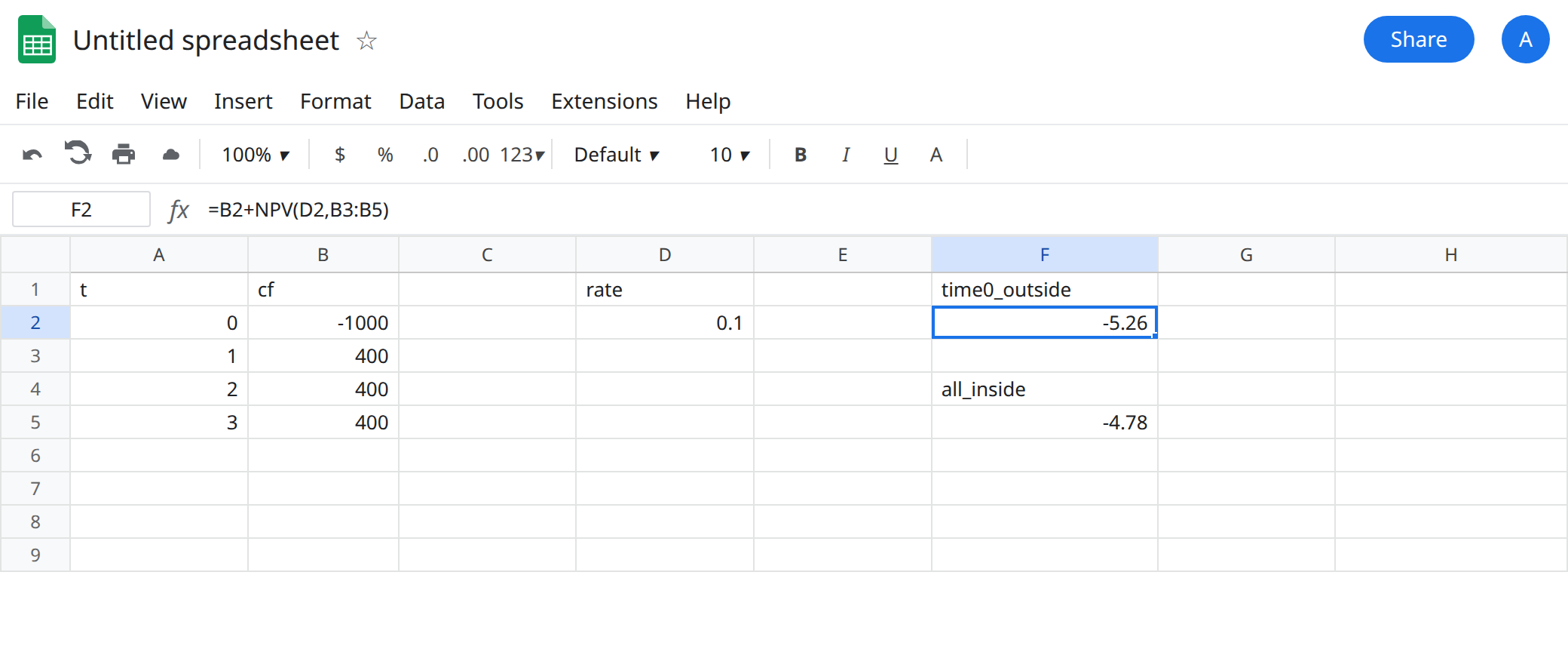
Check the length. =COLUMNS is the wrong size test. Count the cashflows that NPV received: =COUNT(B3:B5) is 3. =COUNT(B2:B5) is 4. If those counts differ by the opening cell, you are about to shift timing again.

Name the header from the formula you actually used. F2 is “outlay at t0 plus NPV of later flows.” F5 is “NPV assuming the outlay is one period from now.” They are both calculable. Only one of them matches column A.

If two NPV cells differ and the only edit was including the first cashflow, the included cell was discounted one extra period. Move that cashflow outside the function.