

HYPERLINK returns #VALUE! for an empty URL or a nested link as the label
Updated
HYPERLINK(url, label) shows label and opens url when you click it. The URL has to be a non-empty text value. An empty string is #VALUE!. The label has to be something Sheets can show as text. Another HYPERLINK in the label is not a text label. The cell is #VALUE!. A URL that is non-empty but not a page (digits, a missing scheme, a space in the middle) can still look like a link and go nowhere useful. That one often has no error triangle.
This page is the empty URL, the nested label, and the link that is not an address. It is not curly quote parse error (#ERROR! before the function runs). It is not VLOOKUP no match except when the URL cell is already #N/A and HYPERLINK only passes that error through. Keep the Google Sheets UI in English.
Recreate it on a blank sheet
Section titled “Recreate it on a blank sheet”- Open a blank spreadsheet. In A1 type
url, B1label. In A2 typehttps://example.com. In B2 typeExample.
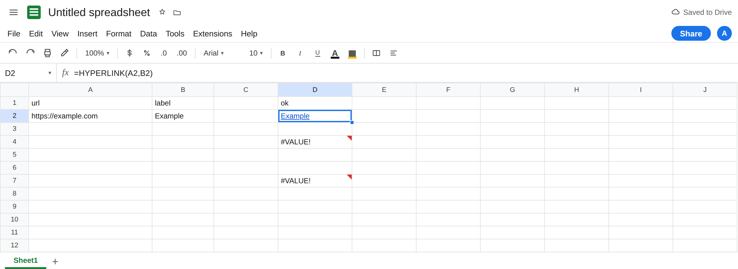
A working link. In D1 type ok. In D2 enter =HYPERLINK(A2,B2). D2 shows Example as a link. Clicking it opens https://example.com. That cell is the control. The label is the second argument. The address is the first. They are not the same string unless you pass the URL twice.
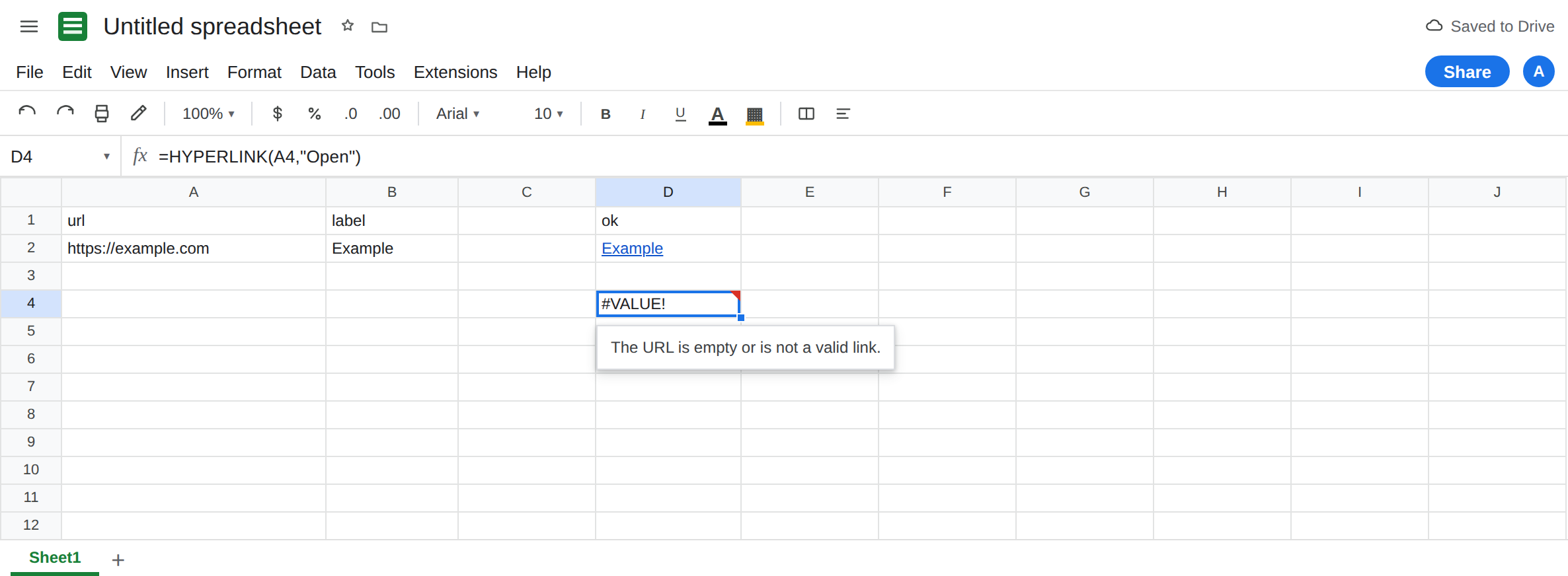
Empty URL. In A4 leave the cell blank. In D4 enter =HYPERLINK(A4,"Open"). The cell shows #VALUE!. The tooltip says the URL is empty or is not a valid link input. Leave D4 broken. A formula that returns "" is the same failure: in A5 enter ="" and in D5 enter =HYPERLINK(A5,"Open"). D5 is #VALUE!. Leave D5 broken.
Nested HYPERLINK as the label. In D7 enter =HYPERLINK(A2,HYPERLINK(A2,"Example")). The outer function wants a label. The inner function returns a link, not a string you can concatenate or display as the label. D7 is #VALUE!. Leave D7 broken. The same trap with concatenation: =HYPERLINK(A2,"See "&HYPERLINK(A2,"help")). The & cannot join text to a hyperlink value. #VALUE!. Leave that in D8 if you entered it.
A label that is a range. In D10 enter =HYPERLINK(A2,B2:B3). Two cells are not one label. The cell errors (#VALUE!). HYPERLINK does not spill a column of links from a two-row range written this way. Leave D10 broken.
No scheme, no triangle. In A12 type example.com with no https://. In D12 enter =HYPERLINK(A12,"Bare"). D12 may show Bare as a link. Clicking it does not open a site, or it treats the text as a relative address inside Sheets. There is often no #VALUE!. In A13 type 123. In D13 enter =HYPERLINK(A13,"Num"). Sheets coerces the number to the text 123. The link address is the digits. It is not https://example.com. Leave D12 and D13 as the quiet bad addresses.
An error in the URL cell passes through. In A15 enter =VLOOKUP(999,A2:B2,1,FALSE). A15 is #N/A. In D15 enter =HYPERLINK(A15,"Missing"). D15 is #N/A, not a link labeled Missing. The lookup failed first. See what #N/A means. Leave D15 broken.
Leave D4, D7, and D10 broken. Leave D2 as the Example link.
What is actually wrong
Section titled “What is actually wrong”- Argument 1 is the address, argument 2 is what the cell displays. Omitting argument 2 displays the URL itself:
=HYPERLINK(A2)showshttps://example.comand still links. That form is legal. It is not how you set a friendly label. The friendly label is D2. - Empty text is not “no link, show the label.”
HYPERLINKrefuses to build a link with no URL. D4 and D5. A space" "can be non-empty and still not be an address. Trim imported URLs.TRIMdoes not addhttps://. - The label is evaluated as a value for display. A nested
HYPERLINK, a range, or an array is#VALUE!. Build the label with text functions (&,TEXT) and pass the finished string. Do not pass a link object. - A curly quote inside the formula, pasted from a doc, is
#ERROR!Formula parse error. The function never ran. See curly quote parse error. D4 is#VALUE!after a successful parse. - Put
IFoutside the call when the URL may be blank:=IF(A4="","",HYPERLINK(A4,"Open")). Do not feed""intoHYPERLINKand then catch it.
Write one HYPERLINK per row. ARRAYFORMULA down a column does not reliably make every row clickable.
Leave D4 and D7 broken.
Text URL, text label. Keep D2: =HYPERLINK(A2,B2). If the URL is missing, keep the link out of the cell: in D17 enter =IF(A4="","",HYPERLINK(A4,"Open")). D17 is blank because A4 is blank. It is not #VALUE!. When A4 later holds https://example.com, change the IF to look at A2 or type the URL into A4. Do not point D17 at A4 and also expect a link while A4 is empty.
One link, one label string. The label is "Example" or B2, not HYPERLINK(...). If you need two addresses, use two cells. Do not nest them.
Put the scheme on quiet failures. D12 should be =HYPERLINK("https://"&A12,"Bare") only when A12 is a host with no scheme. Do not prepend https:// to a cell that already has it (https://https://example.com). Check LEFT(A2,8).
Do not wrap D4 in IFERROR. You cannot tell an empty URL from a nested label. See IFERROR vs IFNA. IFNA would only hide D15’s lookup miss.
If HYPERLINK is #VALUE!, the URL is empty or the label is not text (often a second HYPERLINK). If the cell looks like a link and the browser does nothing, the address has no scheme or is not a URL. D2 is the pattern: a full https string, and a label that is only text.