Merged cells make VLOOKUP and SUMIF see only the first cell

A merged range displays one value across several cells. Sheets stores that value in the top-left cell only. The other cells in the merge are empty. VLOOKUP, SUMIF, COUNTIF, and QUERY read cells, not the painted rectangle. A label that looks like it covers three qty rows is one label and two blanks. The lookup does not “see” the merge.

This page is that gap. It is not VLOOKUP no match (the key is absent, or it is text versus a number). It is not CHAR(160) blanks (an invisible character). The empty cells here are truly empty. Keep the Google Sheets UI in English.

Recreate it on a blank sheet

1. Open a blank spreadsheet. In A1 type dock. In B1 type qty. You are about to merge the dock label on purpose so the bug is visible.

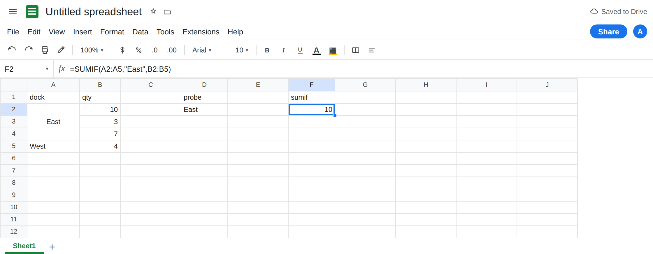
Merge, then type once. Select A2:A4. Format → Merge cells → Merge vertically. With A2:A4 still selected, type East and press Enter. The word sits across three rows. In B2 type 10. B3 type 3. B4 type 7. In A5 type West (do not merge). B5 type 4.

Prove where the text lives. In D1 type probe. In D2 enter =A2. D2 is East. In D3 enter =A3. D3 is blank. In D4 enter =A4. D4 is blank. =COUNTA(A2:A4) is 1. =ISBLANK(A3) is TRUE. The merge is a display. A3 and A4 have no dock.

SUMIF counts one row. In F1 type sumif. In F2 enter =SUMIF(A2:A5,"East",B2:B5). F2 is 10. The eye says East is 10+3+7. The function added B2 only, because A3 and A4 are not East. Leave F2 as 10. That number is the bug, and it has no error triangle.

VLOOKUP returns the first qty. In F4 enter =VLOOKUP("East",A2:B5,2,FALSE). F4 is 10. It found A2. It does not add the rows underneath a merge. There is no #N/A, because the first cell matched.

QUERY sees the same hole. In H1 enter =QUERY(A1:B5,"select A, sum(B) where A = 'East' group by A",1). The spill total is 10, or the where-clause drops the blank rows before the sum. It will not become 20 while A3 and A4 are empty. If the query errors on quotes, this locale’s string rules are QUERY string quotes. The merge is still the data bug.

A lookup aimed at a covered row. In F6 enter =VLOOKUP(A3,A2:B5,2,FALSE). A3 is blank, so the lookup key is blank. You get #N/A or a match on another blank, not the East qty of 3. The row looks labeled. The key cell is empty.

Leave the merge in place. Leave F2 as 10.

What is actually wrong

• Merge writes the value to the upper-left cell and clears the rest. Filtering, sorting, and pivot ranges use those empty cells. The grid can still show East beside B3 because the merge paints over A3. SUMIF does not paint. It compares.
• Sorting a merged column is refused or scrambled. Sheets will warn you that the merge must be unmerged to sort. That warning is the same fact as F2: the column is not three labels.
• Copy-paste of a merged block pastes the merge, not three filled cells. A helper sheet that “looks right” still has blanks. COUNTA is the test, not the screen.
• This is not a type mismatch. East in A2 is text, and "East" is text. F4 found it. See VLOOKUP no match only when COUNTA says the key is present in the cell you think and the lookup still fails.
• A horizontal merge (B2:D2 sharing one qty) stores the number in B2. SUM of B2:D2 adds that number once, not three times. Same rule, other axis.

This is not FILTER no match until you filter on A3. Filtering A2:A5="East" returns one row. The other East qtys never enter the condition.

Fix

Leave F2 in place until the unmerged column sums to 20, so you can see the before and after.

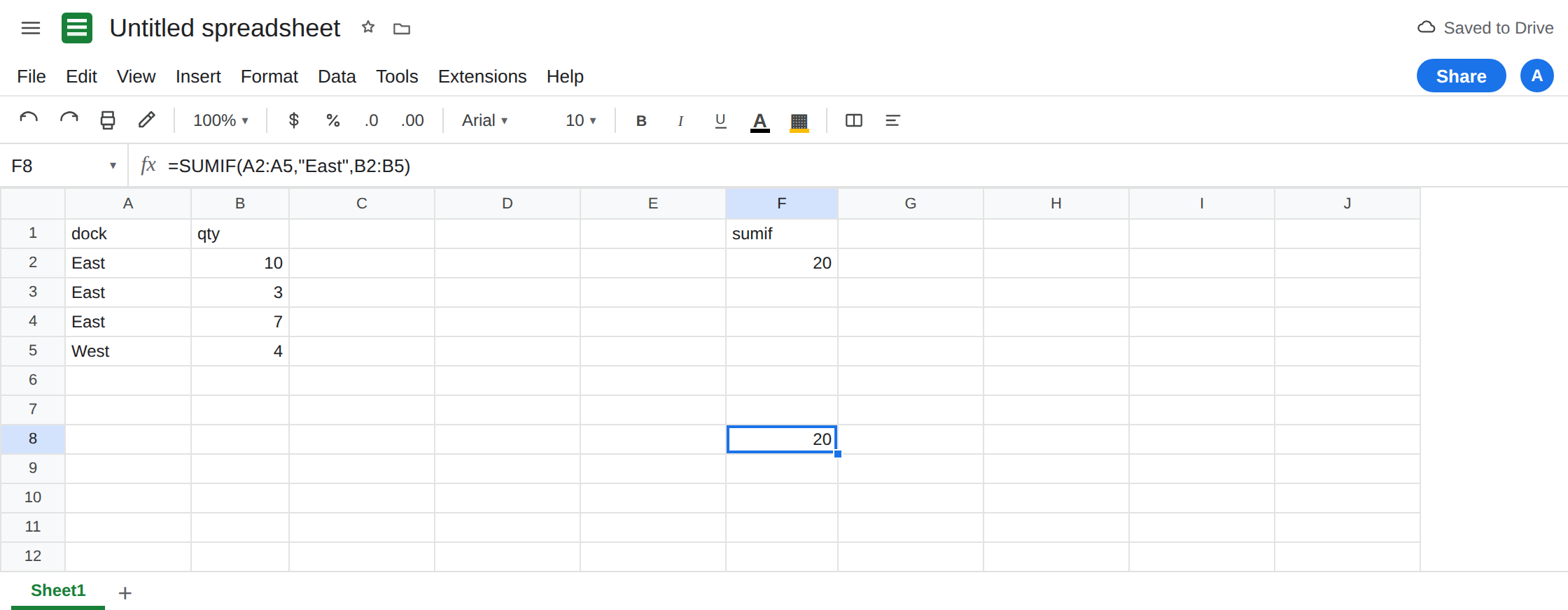
Unmerge and fill the label down. Select A2:A4. Format → Merge cells → Unmerge. A2 still says East. A3 and A4 are empty. Select A2. Drag the fill handle through A4, or enter =A2 in A3 and copy it down, then paste values if you do not want formulas. COUNTA(A2:A4) becomes 3.

Sum again beside the old total. In F8 enter =SUMIF(A2:A5,"East",B2:B5). F8 is 20. F2 is still 10 only if you left a merged copy. On this sheet F2 recalculates to 20 once A3 and A4 contain East. If you need the old wrong total visible, copy F2 to F3 before you unmerge, and paste values.

Do not merge key columns. Merge a title above the table if you need a banner. Do not merge the column VLOOKUP searches or the column SUMIF groups. A pivot wants one label per source row too. GETPIVOTDATA on a pivot built from blanks is GETPIVOTDATA after you have already lost the rows.

Do not wrap F2 in IFERROR. The cell is not an error. It is a small total. See IFERROR vs IFNA.

If the label looks repeated and COUNTA of that block is 1, unmerge and fill. Then run the lookup again.