Fix XLOOKUP return-range spill #REF! in Google Sheets

XLOOKUP can return more than one cell. If result_range is two columns, a hit spills two columns on the formula’s row. If result_range is a block with several rows (one search key matching a vertical return), it spills that shape. #REF! here means that spill would overwrite a filled cell. A one-column return never needs the cell to the right.

This page is XLOOKUP return-array overwrite. It is not XLOOKUP vs VLOOKUP (left lookup, default exact, migration). It is not XLOOKUP #N/A (miss / if_not_found). It is not SORT / UNIQUE spill (different function, same tooltip family). Keep the Google Sheets UI in English.

Recreate it on a blank sheet

1. Open a blank spreadsheet. In A1 type sku, B1 name, C1 bin. A2 101. B2 Widget. C2 A. A3 102. B3 Gadget. C3 B. D1 lookup. D2 101.

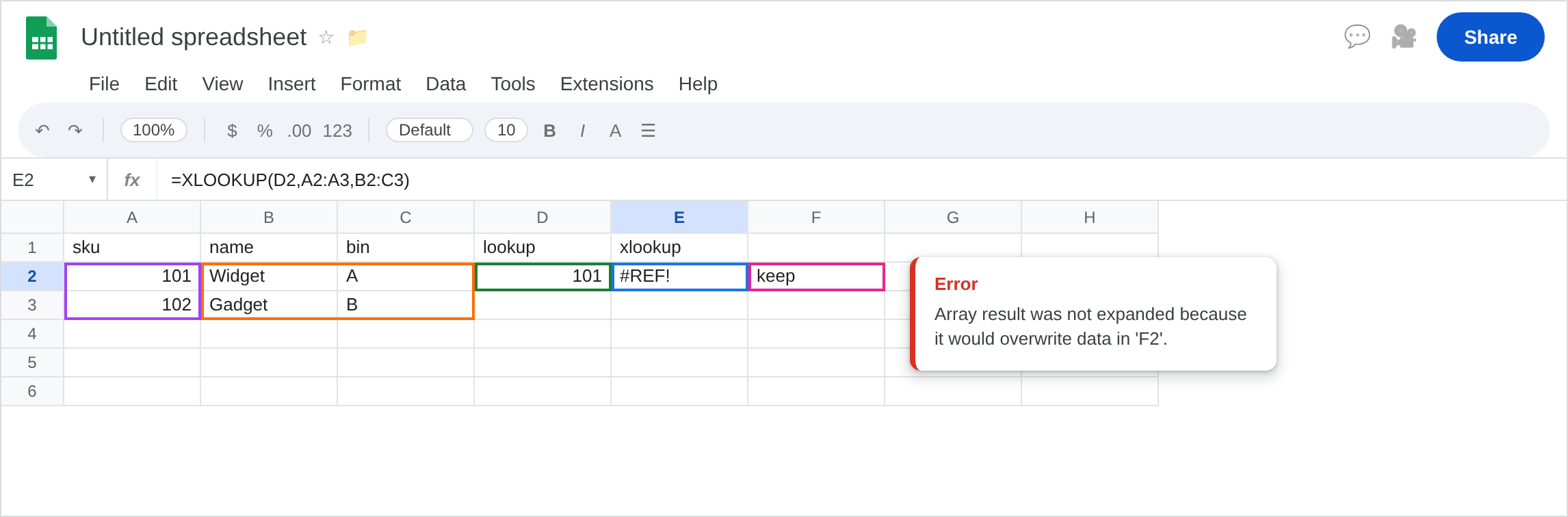
Two-column return, blocked. In E1 type xlookup. In F2 type keep. Leave E2 empty. In E2 enter =XLOOKUP(D2,A2:A3,B2:C3). The cell shows #REF!. The tooltip is Array result was not expanded because it would overwrite data in ‘F2’. A hit on 101 wants E2 = Widget and F2 = A. F2 is occupied. Leave E2 broken.

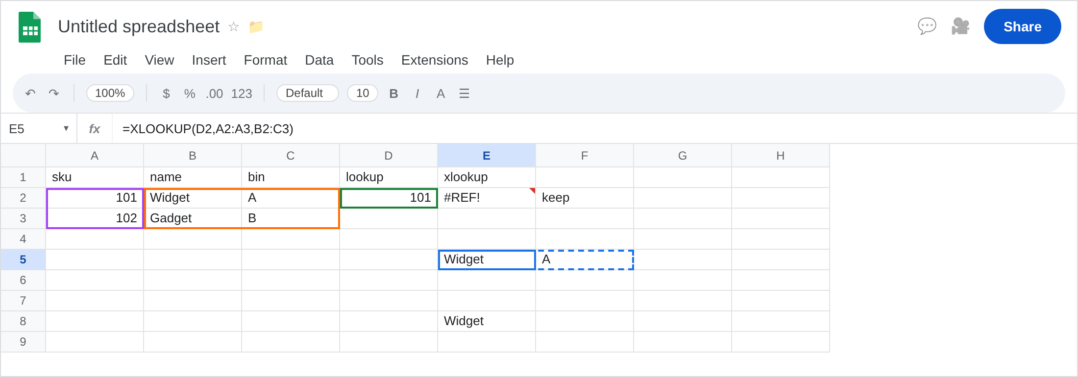
The same return on a clear row. In E5 enter =XLOOKUP(D2,A2:A3,B2:C3). Leave F5 empty. The formula spills Widget / A across E5:F5. That row is the control: two-column result_range, empty path.

One-column return (no right spill). In E8 enter =XLOOKUP(D2,A2:A3,B2:B3). The cell shows Widget only. A value in F8 would not block it.

Miss contrast. In D3 type 999. In E10 enter =XLOOKUP(D3,A2:A3,B2:C3). #N/A, not #REF!. Nothing to spill. That miss is XLOOKUP #N/A. Leave E10 as contrast.

Height mismatch. In E12 enter =XLOOKUP(D2,A2:A3,B2:C2). Lookup is two rows. Return is one row. This errors (size / #N/A / #VALUE! depending on build). Leave E12 broken if it errors. result_range must match lookup_range in the search orientation (same height for a vertical lookup). E2’s ranges match; occupancy is the bug there.

Leave E2 as #REF!. Leave E5 as the working two-column spill. Leave E10 as #N/A.

What is actually wrong

• result_range B2:C3 is names and bins. A match returns that whole row slice. E2 needs two empty cells.
• Occupied F2 blocks the entire result. Sheets does not write Widget into E2 and skip the bin. One #REF!.
• A miss never spills, so it cannot #REF! from occupancy. E10 is #N/A even if F10 is full.
• This is not VLOOKUP’s third-argument index. VLOOKUP(D2,A2:C3,2,FALSE) returns one cell (name) and will not overwrite F2. Migration to XLOOKUP with a wide return is how the spill appears. See XLOOKUP vs VLOOKUP for the migration, then come back here for overwrite.

This is not a deleted reference inside the formula bar. See after you delete. E2 still names B2:C3.

This is not search_mode binary. See XLOOKUP search_mode.

This is not INDEX past the range. See INDEX past range.

Fix

Leave E2, E10, and E12 broken.

Clear the neighbor or move the formula. Keep E5: =XLOOKUP(D2,A2:A3,B2:C3) with F5 empty. Delete keep in F2 only if E2 must stay. Do not wrap E2 in IFERROR. You still have no name/bin pair. See IFERROR vs IFNA.

Need one field? Return one column: keep E8. Two XLOOKUPs (name, then bin) also stay scalars.

Need every match, not one row: =FILTER(B2:C3,A2:A3=D2) — also a spill, also #REF! if blocked. Same occupancy rule.

If #REF! and the formula is XLOOKUP with a multi-column return, look right (or down). If #N/A, the key missed. If one column returns Widget and you expected a bin too, widen result_range and clear the path.

Wide return vs VLOOKUP index vs miss

XLOOKUP + B2:C3 → 2-wide spill. Occupancy #REF! (E2). This page.

VLOOKUP index 2 → scalar name. No F2 spill. Migration is XLOOKUP vs VLOOKUP.

XLOOKUP of 999 → #N/A (XLOOKUP #N/A). if_not_found does not clear a #REF! overwrite. Fix the path, then decide on misses.