XNPV returns an error when dates and amounts differ in length

XNPV(discount, cashflow_amounts, cashflow_dates) discounts each amount from its own date. The two ranges pair by position: amount 1 with date 1. Three amounts and two dates cannot pair. The cell errors. The tooltip is about the ranges, not about the discount rate. A date stored as text is #VALUE! even when the lengths match. A matched schedule with one negative amount and later positive amounts returns a number.

NPV without the X is a different timing rule: the first value inside NPV is end of period 1. That page is NPV timing. A rate that never converges is IRR / XIRR #NUM! and RATE guess. These figures only show pairing. This is not a recommendation to invest or to borrow. Keep the Google Sheets UI in English. Sheet Error is an independent formula-error library, not a Google product.

Recreate it on a blank sheet

1. Open a blank spreadsheet. In A1 type amt, B1 when. A2 -100. A3 60. A4 60. In B2 enter =DATE(2024,1,1). B3 =DATE(2024,7,1). B4 =DATE(2025,1,1). Format B2:B4 as Date. One outflow, two inflows, three dates.

A present value that works. In D1 type xnpv_ok. In D2 enter =XNPV(0.1,A2:A4,B2:B4). The discount is 10% a year, written as 0.1, not as 10. Three amounts, three dates. D2 is a number (negative or positive depending on the spacing; on these dates it is not an error). Format D2 as a number if it looks like a date. That cell is the control: the lengths match and the dates are real serials.

Dates shorter than the amounts. In D4 type short_dates. In D5 enter =XNPV(0.1,A2:A4,B2:B3). Three amounts, two dates. The cell shows #N/A or #VALUE!. The tooltip is about range size. The signs in A2:A4 are already usable. The discount is the same 0.1 that D2 accepted. Leave D5 broken.

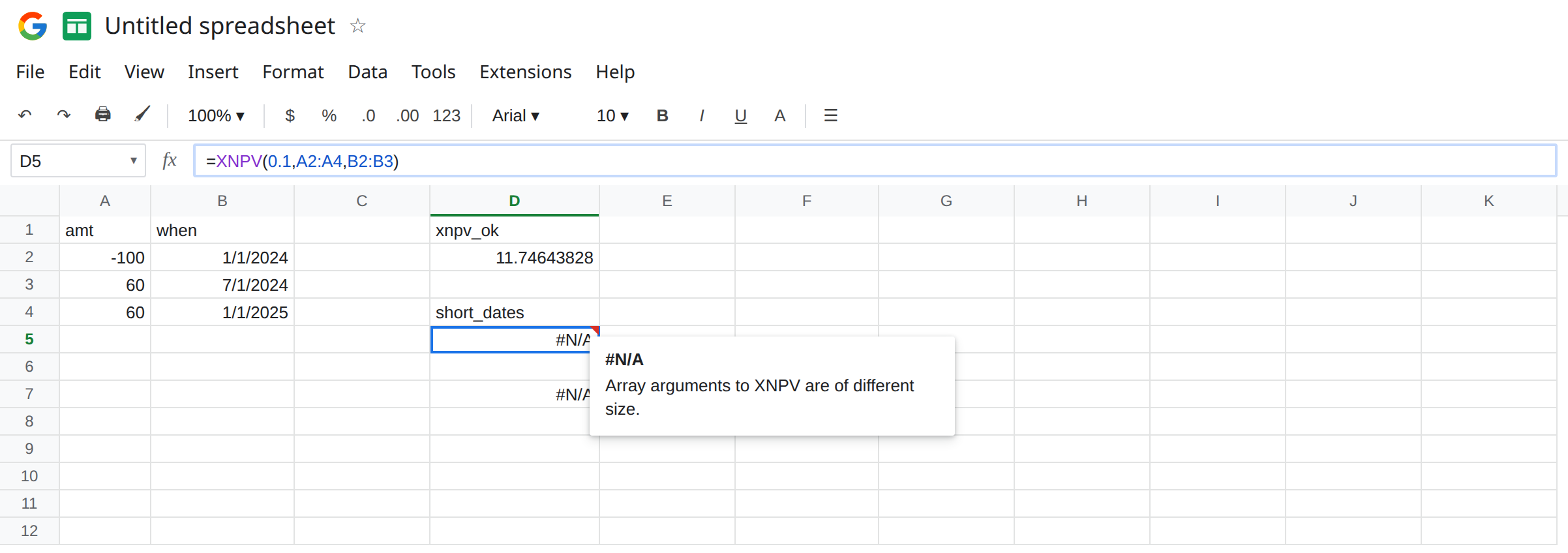
Amounts shorter than the dates. In D7 enter =XNPV(0.1,A2:A3,B2:B4). Two amounts, three dates. The same class of error. Leave D7 broken. Either side can be short.

A date typed as text. In C2 type '1/1/2024 with a leading apostrophe so the cell is text. C3 enter =DATE(2024,7,1). C4 enter =DATE(2025,1,1). =ISTEXT(C2) is TRUE. In F2 enter =XNPV(0.1,A2:A4,C2:C4). Lengths match. C2 is not a date serial. F2 is #VALUE!. See DATEVALUE locale if you meant to parse that string. Leave F2 as #VALUE!. Do not call it a short range.

Discount as a whole number. In F4 enter =XNPV(10,A2:A4,B2:B4). Lengths match. 10 means 1000% a year, not 10%. The cell returns a number, usually a small one, with no triangle. It is not D5. If you wanted 10%, the argument is 0.1 or a cell formatted as percent that contains 0.1. Leave F4 as that number so it is not confused with the size error.

Leave D5 and D7 as the size errors. Leave F2 as #VALUE!. Leave D2 as a number.

What is actually wrong

• XNPV lines the ranges up from the top. It does not match dates to amounts by a key, and it does not drop a blank to “make the lengths fit.” A blank row in the middle of one range and not the other changes the count or shifts the pairs.
• The error on D5 is the counts. Changing 0.1 to 0.08 will not clear it. Adding the third date will.
• Text that looks like a date is still text. ISTEXT or ISNUMBER on the date cell tells you which. ISNUMBER of a real DATE result is TRUE. F2 fails ISNUMBER on C2.
• The first date is the start of the schedule. Later dates should not fall before it. A date earlier than B2 can be #NUM! even when the lengths match. That is a different failure from D5. Keep B2 as the earliest date on this sheet so the control stays a number.
• XNPV of a discount equal to XIRR on the same amounts and dates is 0. That identity needs the same paired ranges. It does not need a shorter date list. Sign rules for the rate itself live on IRR / XIRR #NUM!.

This is not NPV(0.1,A2:A4), which ignores column B and discounts by period index. See NPV timing. If D2 and that NPV disagree, the dates are doing real work. That disagreement is not the size bug.

This is not PMT’s negative payment. See PMT sign. A2 is negative because it is money out. The error in D5 is length.

Fix

Leave D5, D7, and F2 broken.

Use the same rows on both ranges. Keep D2: =XNPV(0.1,A2:A4,B2:B4). If you insert a cashflow, insert a date on that same row and extend both ranges together.

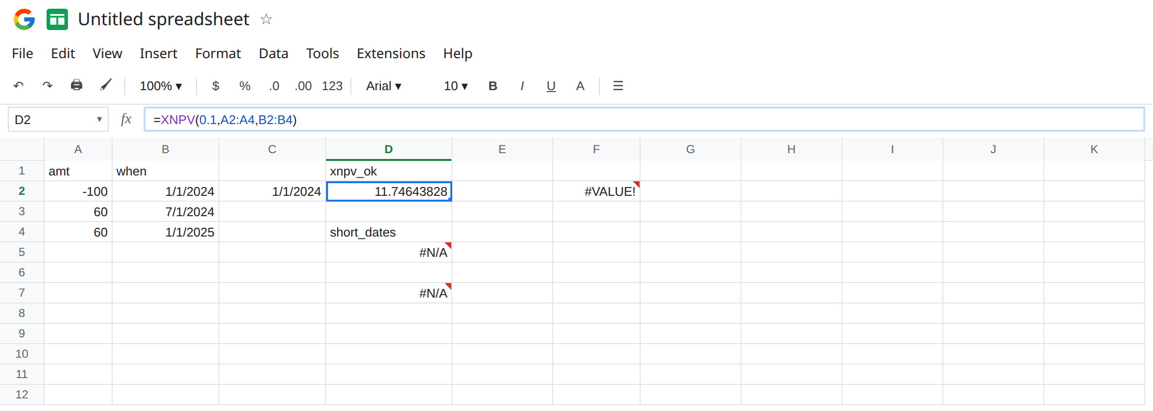
Replace text dates. C2 should be =DATE(2024,1,1) or DATEVALUE of a string this locale accepts. Then point XNPV at that column. Do not pass the apostrophe-text cell.

Write the discount as a fraction. 0.1 for 10 percent. F4’s 10 is a different problem, and it still calculates.

Do not wrap D5 in IFERROR and report a present value of 0. A short date list has no XNPV. See IFERROR vs IFNA. IFNA might hide a #N/A size error and would not explain it.

If XNPV errors and the tooltip is about size, count dates against amounts (D5, D7). If it is #VALUE! and a date cell is text, convert the date (F2). If it is a number you did not expect, check that 0.1 was not typed as 10, and check that the first date is the earliest. NPV is the function that does not take dates.

Length vs text vs the rate

D2 pairs three and three and returns a number at discount 0.1. D5 and D7 are short on one side. F2 is #VALUE! because C2 is text. F4 is a number at discount 10, which is not 10 percent. None of those is IRR failing to converge.