ISERROR, ISNA, and ISERR each miss a different error

ISERROR, ISNA, and ISERR all return TRUE or FALSE. They do not return the same TRUE. ISNA is TRUE only for #N/A. ISERR is TRUE for every error except #N/A. ISERROR is TRUE for every error, including #N/A. A sheet that uses ISERR to “catch lookup misses” prints FALSE on a real #N/A. A sheet that uses ISNA to “catch bad math” prints FALSE on #DIV/0! and #VALUE!. The formula parsed. The flag is the wrong flag.

IFERROR and IFNA replace the error with another value. These three functions only test. The wrapper comparison is IFERROR vs IFNA. What #N/A means on a lookup is what #N/A means. Keep the Google Sheets UI in English. Sheet Error is an independent formula-error library, not a Google product.

Recreate it on a blank sheet

1. Open a blank spreadsheet. In A1 type sku, B1 name. A2 101, B2 Widget. D1 lookup. D2 999. That sku is not in column A.

Three different errors. In E1 type na. In E2 enter =VLOOKUP(D2,A2:B2,2,FALSE). E2 is #N/A. In F1 type div. In F2 type 0. In F3 enter =1/F2. F3 is #DIV/0!. In G1 type val. In G2 enter =10+"pcs". G2 is #VALUE!. Leave E2, F3, and G2 broken. They are the three inputs. See divide by zero and wrong type if you want the primer for F3 and G2. Do not fix them on this page.

ISNA on all three. In I1 type isna. In I2 enter =ISNA(E2). I2 is TRUE. In I3 enter =ISNA(F3). I3 is FALSE. In I4 enter =ISNA(G2). I4 is FALSE. #DIV/0! and #VALUE! are errors. ISNA does not see them.

ISERR on all three. In J1 type iserr. In J2 enter =ISERR(E2). J2 is FALSE. The cell you tested is #N/A, and ISERR is defined to ignore #N/A. In J3 enter =ISERR(F3). J3 is TRUE. In J4 enter =ISERR(G2). J4 is TRUE. This is the wrong pick for a lookup: the miss looks like “not an error.”

ISERROR on all three. In K1 type iserror. In K2 enter =ISERROR(E2). K2 is TRUE. In K3 enter =ISERROR(F3). K3 is TRUE. In K4 enter =ISERROR(G2). K4 is TRUE. In K5 enter =ISERROR(101). K5 is FALSE. A number is not an error. ISERROR does not mean “this cell looks suspicious.”

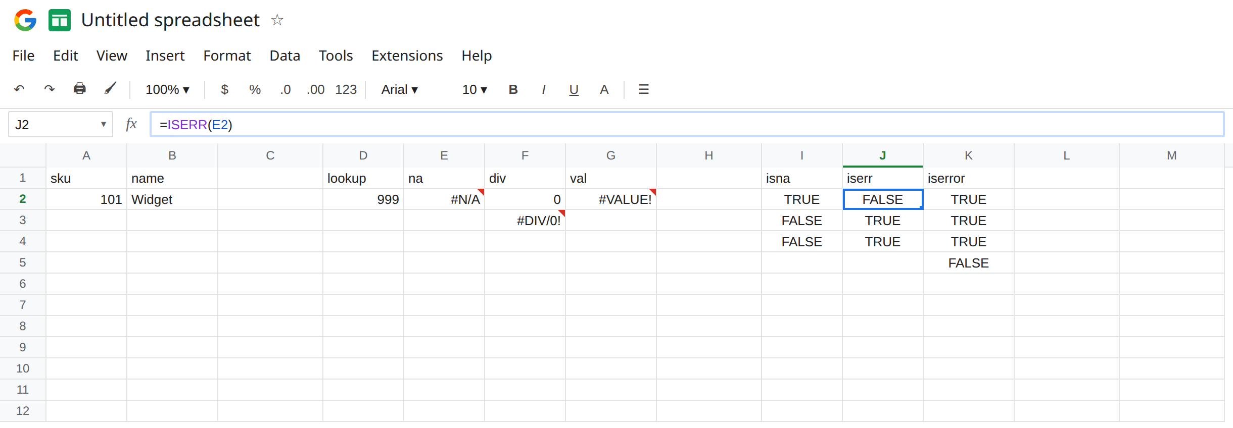
Leave J2 as FALSE on a real #N/A. Leave I3 as FALSE on a real #DIV/0!. =ISNA(101) is FALSE. An ordinary value is not #N/A.

What is actually wrong

• ISNA answers one question: is this #N/A? A VLOOKUP miss is yes. A zero divisor is no. A wrong type is no. A successful lookup of 101 is no.
• ISERR answers a different question: is this an error other than #N/A? The lookup miss is no. That FALSE is easy to read as “the sku was found.” It was not. E2 is still #N/A.
• ISERROR answers the wide question. It is the right test when any error should take the same branch, and the wrong test when a #REF! from a bad index should stay visible while a miss becomes "none". Hiding every error is IFERROR hides cause.
• The functions do not change the cell they test. E2 stays #N/A while I2 is TRUE. People copy ISERR into a column of flags and then filter where the flag is FALSE, which keeps the misses in the “good” set.
• IF(ISERR(E2),"bad",E2) returns #N/A, not "bad", because the condition is FALSE and the false branch is the error itself. The flag did not catch it, so the error comes back.

This is not IFNA(E2,"none"). IFNA replaces #N/A and lets #DIV/0! through. ISNA only reports. See IFERROR vs IFNA.

This is not ERROR.TYPE, which turns the error into a number you can filter. That map is ERROR.TYPE codes. ISERROR cannot tell #DIV/0! from #VALUE!. Both are TRUE.

Fix

Leave E2, F3, G2, J2, and I3 as they are so the wrong flags stay on the sheet.

Match the test to the error you mean. For the lookup only, use ISNA. In L2 enter =IF(ISNA(E2),"missing",E2). L2 is missing. In L3 enter =IF(ISNA(F3),"missing",F3). L3 is still #DIV/0!. That is what you want if a zero divisor should not be labeled “missing.”

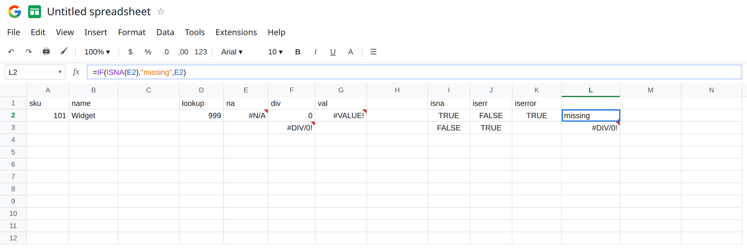
For any error, use ISERROR, and know what you hid. =IF(ISERROR(F3),"bad",F3) is bad. The same formula on E2 is also bad. You can no longer see which error it was. Prefer IFNA for lookups and leave other errors alone.

Do not use ISERR as a synonym for ISERROR. J2 is the proof. If the branch should run on #N/A, ISERR will not run it.

Do not wrap the flag in IFERROR. ISNA of an error is TRUE or FALSE, not an error of its own. IFERROR around J2 would not turn FALSE into TRUE.

If the flag is FALSE and the cell you tested still shows an error, you picked the test that excludes that error. #N/A needs ISNA or ISERROR. #DIV/0! and #VALUE! need ISERR or ISERROR. ISNA will not see them.

Which test sees which error

Cell	Error	ISNA	ISERR	ISERROR
E2	#N/A	TRUE	FALSE	TRUE
F3	#DIV/0!	FALSE	TRUE	TRUE
G2	#VALUE!	FALSE	TRUE	TRUE
A2	number 101	FALSE	FALSE	FALSE

ISERR on E2 is the miss this page exists for. ISNA on F3 is the other miss. ISERROR sees both and also sees a bad index #REF!, so it is a coarse test, not a lookup test.