Fix YEARFRAC #NUM! in Google Sheets (basis out of range)

YEARFRAC(start_date, end_date, [basis]) returns the fraction of a year between two dates. basis is the day-count convention: 0 US 30/360 (default), 1 actual/actual, 2 actual/360, 3 actual/365, 4 European 30/360. #NUM! here means basis is outside 0–4 (negative, 5, 99). A reversed date pair usually still returns a negative fraction — that is not this #NUM!. DATEDIF is the function that refuses reversed dates.

This page is YEARFRAC basis. It is not DATEDIF #NUM! (end before start). It is not out of domain (SQRT(-1)). It is not WORKDAY #NUM!. Keep the Google Sheets UI in English. Format the result as Number.

Recreate it on a blank sheet

1. Open a blank spreadsheet. In A1 type start, B1 end. In A2 enter =DATE(2024,1,1). In B2 enter =DATE(2024,7,1). Format as Date. Half a calendar year, give or take the basis.

Working Actual/Actual. In D1 type basis1. In D2 enter =YEARFRAC(A2,B2,1). The cell shows a fraction near 0.5 (182 / 366 in 2024, a leap year). That row is the control.

Default 30/360. In D4 enter =YEARFRAC(A2,B2,0) or =YEARFRAC(A2,B2). Close to 0.5 as well (180/360). Different convention, still legal.

Basis 5. In F1 type basis5. In F2 enter =YEARFRAC(A2,B2,5). The cell shows #NUM!. There is no basis 5. Leave F2 broken.

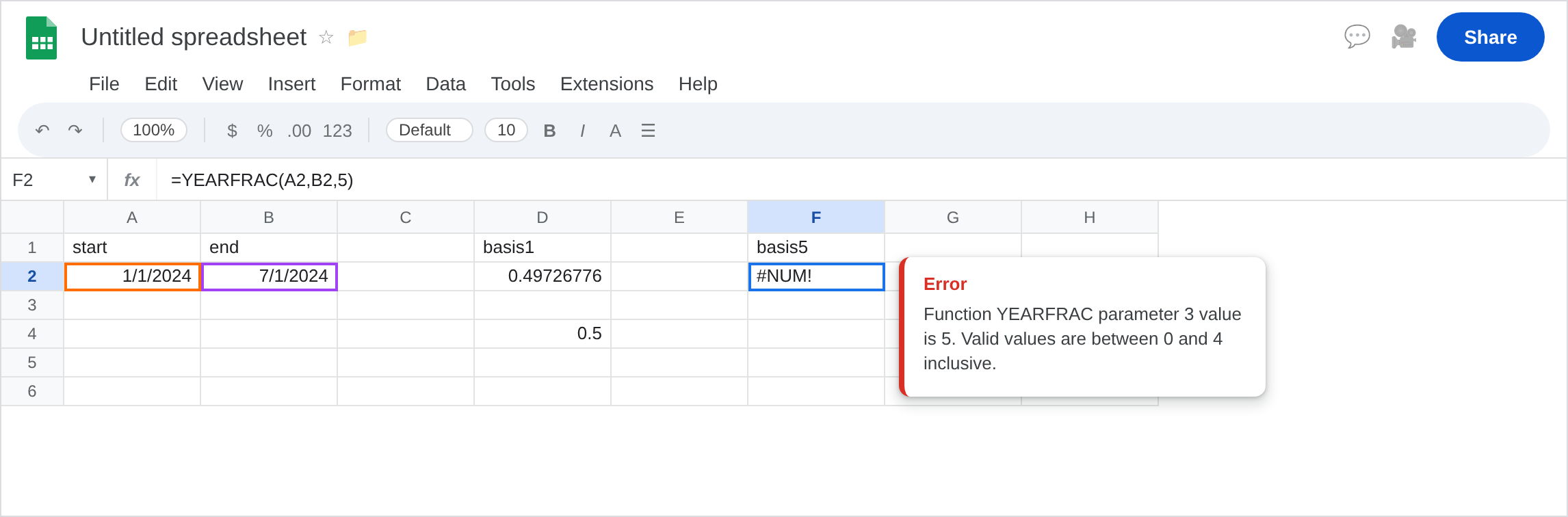
Basis 99. In F4 enter =YEARFRAC(A2,B2,99). #NUM!. Leave F4 broken.

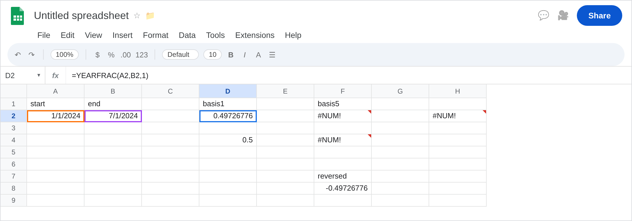
Reversed dates (not this error). In F7 type reversed. In F8 enter =YEARFRAC(B2,A2,1). The cell is about -0.5, not #NUM!. Leave F8 as the signed fraction. =DATEDIF(B2,A2,"D") on that order would be the other page’s #NUM! if you swapped DATEDIF’s arguments the same way — here YEARFRAC cooperates.

DATEDIF contrast. In H2 enter =DATEDIF(B2,A2,"D"). End (Jan 1) before start (Jul 1) in DATEDIF’s slots → #NUM!. Leave H2 as the contrast. Do not copy a DATEDIF swap onto F2. F2’s dates are already in the right order; the basis is illegal.

Leave F2 and F4 broken. Leave D2 as the working fraction. Leave F8 negative.

What is actually wrong

• basis is an integer 0–4. It is not a year, not a WEEKDAY type, not a WORKDAY.INTL weekend code. 5 and 99 are #NUM!.
• Omitting basis is 0 (US 30/360), not “actual.” Accrual sheets that assume actual/actual must pass 1.
• Leap years change basis 1. 2024-01-01 to 2024-07-01 is 182/366, not 181/365. Basis 3 uses 365 in the denominator even in a leap year. The numbers disagree on purpose.
• Negative YEARFRAC means the dates are swapped. That is information, not #NUM!. Use ABS if you want magnitude.
• Text dates go through locale parsing on some paths and #VALUE! on others. This recreate uses DATE so the only red cell is basis.

This is not DATEDIF "MD" leftover bugs. See DATEDIF #NUM!.

This is not WEEKDAY type 99. See WEEKDAY #NUM!. Same 99, different argument.

This is not EOMONTH months overflow. See EOMONTH #NUM!.

Fix

Leave F2, F4, and H2 broken.

Pass basis 0–4. Keep D2: =YEARFRAC(A2,B2,1) for actual/actual. 30/360 US: 0. Actual/365: 3. European 30/360: 4.

If you meant DATEDIF days: =DATEDIF(A2,B2,"D") with the earlier date first — not YEARFRAC(...,5).

If you wanted a positive fraction regardless of order: =ABS(YEARFRAC(A2,B2,1)), or IF(B2>=A2,YEARFRAC(A2,B2,1),YEARFRAC(B2,A2,1)).

Do not wrap F2 in IFERROR so an illegal basis prints 0. That looks like “zero years.” See IFERROR vs IFNA.

If #NUM! and the third argument is 5 or 99, this is the page. If #NUM! and the formula is DATEDIF, leave. If the fraction is negative, swap dates or take ABS. If two legal bases disagree, read 30/360 vs actual — both can be right.

Basis 5 vs DATEDIF reverse vs 30/360 vs actual

YEARFRAC basis 5 → #NUM! (F2).

DATEDIF reverse → #NUM! (H2). Different function.

YEARFRAC reverse → negative (F8). Same function, not an error.

Default 0 vs 1 is a convention choice, not a red triangle. Pick 1 when the calendar day count should win; pick 0 or 4 when the sheet is 30/360 interest math.