RATE returns #NUM! when the guess does not converge

RATE(number_of_periods, payment, present_value, [future_value], [end_or_beginning], [rate_guess]) solves for the interest rate per period. It searches from a guess. The default guess is 0.1 (10% per period). A guess that never lands is #NUM!. A payment and a present value with the same sign often have no rate at all, and every guess is #NUM!. The guess is a decimal per period, not a percent already scaled, and not an annual rate you forgot to match to the payment.

IRR has the same kind of guess. See IRR / XIRR #NUM!. The payment’s sign is PMT sign. These figures only show convergence. This is not lending advice. Keep the Google Sheets UI in English. Sheet Error is an independent formula-error library, not a Google product.

Recreate it on a blank sheet

1. Open a blank spreadsheet. In A1 type nper, B1 pmt, C1 pv. A2 12. B2 -100. C2 1000. Twelve periods, a payment of 100 out, a present value of 1000 in. Opposite signs.

No guess. In E1 type rate_ok. In E2 enter =RATE(A2,B2,C2). E2 is about 0.02923 (about 2.92% per period). Format E2 as a percent if you want to read 2.92%. There is no triangle. The default guess 0.1 was close enough. That cell is the control. Check the payment that belongs to it: =PMT(E2,A2,C2) is -100, the same cash you started with, once you format it. Signs in, rate out.

A guess that does not converge. In E4 type guess5. In E5 enter =RATE(A2,B2,C2,0,0,5). The fourth argument is future value 0. The fifth is 0 (payment at end of period). The sixth is the guess 5, which means 500% per period, not 5%. The cell shows #NUM!. The cashflows are the ones that already solved in E2. The search from 5 does not arrive. Leave E5 broken.

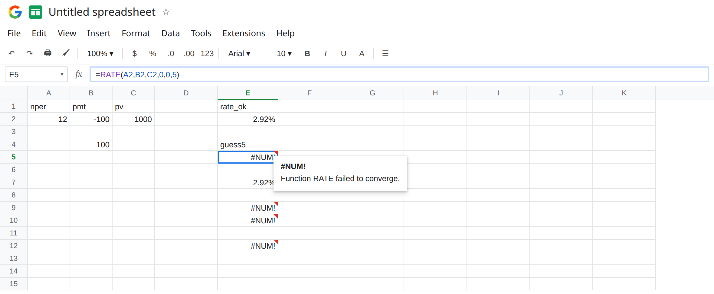
Guess of 5 percent, written wrong. In E7 enter =RATE(A2,B2,C2,0,0,0.05). E7 is about 2.92%, the same as E2. 0.05 is a legal guess (5% per period) near the answer. The bug in E5 is the scale of 5, not the presence of a sixth argument.

Same sign. In B4 type 100 (no minus). In E9 enter =RATE(A2,B4,C2). Payment in and present value in. The cell shows #NUM!. There is no rate that makes a string of inflows, with a zero future value, balance. In E10 enter =RATE(A2,B4,C2,0,0,0.01). Still #NUM!. A closer guess does not create a root that is not there. Leave E9 and E10 broken.

A guess at or below −100%. In E12 enter =RATE(A2,B2,C2,0,0,-1). A rate of -1 or below breaks the compounding term. #NUM!. Leave E12 broken. The solvable series is still E2.

Leave E5, E9, and E12 as #NUM!. Leave E2 as the rate near 2.92%.

What is actually wrong

• The sixth argument is optional. Omit it until the no-guess formula works. If E2 is a rate and E5 is #NUM!, delete the guess or replace 5 with a decimal near E2 (0.03, not 5 and not 3).
• Same-sign payment and present_value, with future value 0, is #NUM! for a mathematical reason. Flipping the guess does not fix B4. Flip the payment’s sign only when that cash really leaves the account. See PMT sign. PMT of a positive present value is negative. Feeding that negative payment back into RATE is E2. Feeding ABS of it is E9.
• Future value and the timing flag sit before the guess. =RATE(A2,B2,C2,5) passes 5 as the future value, not as the guess. The formula can return a rate (a different problem: money left over) with no #NUM!. To pass a guess you must pass future value and end-or-beginning too, which is what E5 does. People insert ,5 at the end of a three-argument call and think they set the guess.
• end_or_beginning is 0 or 1. It is not the guess. A 1 in the sixth slot is a guess of 100% per period, which may #NUM! or may converge to a wrong search. Count the commas.
• #NUM! here is not SQRT(-1). See out of domain. The inputs are ordinary loan numbers. The solver did not finish, or no rate exists.

This is not XNPV range length. See XNPV dates. RATE does not take a date column. Periods are assumed equal.

This is not a divide by zero. See divide by zero. E5 is #NUM!.

Fix

Leave E5, E9, and E12 broken.

Use the no-guess result. Keep E2: =RATE(A2,B2,C2). If you must pass a guess, use a decimal per period near the rate you expect. In G2 enter =RATE(A2,B2,C2,0,0,0.03). G2 matches E2. Do not pass 5 and do not pass 3 meaning “3 percent.”

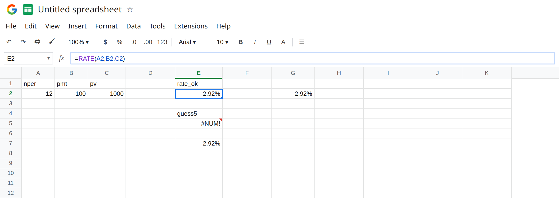
Put the signs on opposite sides of zero. Money in and money out. B2 stays -100 if C2 stays 1000. If both should be positive because you stored the payment as a positive bill, make the present value negative instead. Do not make them match.

Count arguments before you add a guess. Three arguments when the defaults are fine. Six when you really have a future value, a timing flag, and a guess. =RATE(A2,B2,C2,0,0,0.03) is the six-argument form of G2.

Do not wrap E5 in IFERROR and show 0.1. A guess that failed is not “10% by default.” See IFERROR vs IFNA. IFNA does not catch #NUM!.

If RATE is #NUM!, delete the guess and look at E2. If the no-guess call is also #NUM!, check that payment and present value have opposite signs (E9). If a trailing 5 was meant as 5 percent, it is either a future value or a 500% guess, depending on how many arguments you already passed.

Guess vs signs

E2, no guess, opposite signs: about 2.92% per period. E7, guess 0.05: the same rate. E5, guess 5: #NUM!. E9, payment 100 and present value 1000: #NUM! even with a small guess. E12, guess -1: #NUM!. PMT of E2 over 12 periods on 1000 returns -100.