LOOKUP’s result vector is positional, and the search vector has to be sorted

LOOKUP(search_key, search_vector, result_vector) does not take a column index. The third argument is a second range, paired with the search vector by position: row 1 with row 1, row 2 with row 2. The search vector must be sorted ascending. The match is always approximate. If the key is missing, you get the largest search value that is still smaller, and the result cell beside that position. Nothing in the formula says “approximate.” A result vector with fewer rows than the search vector is #N/A. A result vector that starts on the wrong row is the same length and still the wrong names, with no error.

The sorted quantity-break case, where approximate is what you wanted, is LOOKUP approximate. The one-range array form, which picks a direction from the shape, is LOOKUP array form. Exact XLOOKUP is XLOOKUP #N/A. Keep the Google Sheets UI in English. Sheet Error is an independent formula-error library, not a Google product.

Recreate it on a blank sheet

1. Open a blank spreadsheet. In A1 type qty, B1 name. A2 40, B2 Sofa. A3 10, B3 Desk. A4 30, B4 Lamp. A5 20, B5 Chair. The qty column is not sorted. Desk is the name beside 10. Chair is beside 20. Lamp is beside 30. Sofa is beside 40.

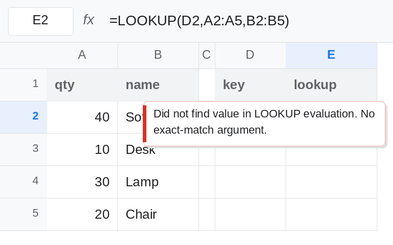
Unsorted search, no triangle. In D1 type key. D2 25. In E1 type lookup. In E2 enter =LOOKUP(D2,A2:A5,B2:B5). E2 returns a name, or #N/A. Whichever name appears, it is not a break price you can defend. The function still assumed A2:A5 was ascending. 25 is not even in the column. There is no exact-match switch to make this #N/A on purpose. Leave E2 as that result and do not ship it.

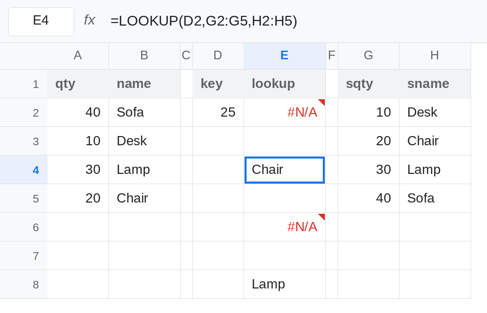
The same key on a sorted search. In G1 type sqty, H1 sname. G2 10, H2 Desk. G3 20, H3 Chair. G4 30, H4 Lamp. G5 40, H5 Sofa. In E4 enter =LOOKUP(D2,G2:G5,H2:H5). E4 is Chair. The largest sorted qty that is still <= 25 is 20. This is the only LOOKUP result on the sheet that matches the break rule. It is still approximate: 25 is not a qty. Leave E4 as Chair.

A shorter result vector. In E6 enter =LOOKUP(D2,G2:G5,H2:H4). The search vector is four rows. The result vector is three. E6 is #N/A. The key and the sort are fine. The vectors do not pair. Leave E6 broken.

Same length, shifted start. In E8 enter =LOOKUP(20,G2:G5,H3:H6). Both vectors are four cells. H3:H6 is Chair, Lamp, Sofa, and a blank. The blank is H6. 20 is an exact key and sits in G3, the second search cell, so LOOKUP returns the second result cell, H4, which is Lamp. The name beside 20 in the sorted table is Chair, in H3. The formula never checked that H3:H6 was the name column. It zipped by position. Leave E8 as Lamp. No triangle.

Exact functions on the unsorted block. In E10 enter =XLOOKUP(25,A2:A5,B2:B5,"missing"). E10 is missing. 25 is not a qty. In E11 enter =XLOOKUP(10,A2:A5,B2:B5,"missing"). E11 is Desk, the name actually beside 10, and the search column did not need to be sorted. Leave E10 as missing.

Leave E2 unused as a price. Leave E4 as Chair. Leave E6 as #N/A. Leave E8 as Lamp.

What is actually wrong

• The third argument is not VLOOKUP’s column index. It is a parallel vector. Position 2 in the search vector returns position 2 in the result vector. E8 proves the pairing with a shifted window: exact key, wrong name, no error.
• Approximate match is not optional. On a sorted vector, 25 returns the 20 row, Chair. That can be what a price break means. It is never what a sku lookup means. See LOOKUP approximate for the break table written out.
• Unsorted search does not become exact and does not reliably become #N/A. E2 is not Desk just because Desk is the 10 row. Sort the search vector, or stop using LOOKUP.
• A shorter result vector is the #N/A case. E6. A longer result vector ignores the extra cells and still pairs from the top. Same length is not the same as “the column next to the key.”
• XLOOKUP takes the same two ranges and, by default, requires an exact key. E10 and E11. It does not need the qty column sorted.

This is not VLOOKUP wrong row from a TRUE fourth argument, except that both are approximate. VLOOKUP’s third argument is an index into one table. LOOKUP’s third argument is a separate range that can drift, which is E8.

Fix

Leave E2 unsorted. Leave E6 broken. Leave E8 as the shifted Lamp.

Price breaks, both vectors sorted and aligned. Keep E4: =LOOKUP(D2,G2:G5,H2:H5). G2:G5 must stay ascending. H2:H5 must be the names of those same rows, starting on the same first row. If 100 should not silently return Sofa, LOOKUP will not tell you. Use a ceiling test, or use an exact function.

Sku or any exact key. Use E11’s shape: =XLOOKUP(10,A2:A5,B2:B5,"missing"). Unsorted A2:A5 is allowed. A missing key is the fourth argument, not a neighbor. See XLOOKUP #N/A.

If the result must be #N/A below the first break, that part LOOKUP already does on a sorted vector. =LOOKUP(5,G2:G5,H2:H5) is #N/A, because nothing is <= 5. Do not cite that #N/A as evidence the function is exact. 25 is still Chair.

Do not wrap E2 in IFERROR. A wrong name is not an error. See IFERROR vs IFNA.

If LOOKUP returns a name for a key that is not in the search column, it approximated. Sort the search vector and align the result vector, or switch to XLOOKUP. If the vectors differ in length, the #N/A is the length, not the key. If they match in length and the name is the neighbor’s name, the result range starts on the wrong row.