CHOOSEROWS returns an error for 0, a bad negative, or a mixed index list

CHOOSEROWS picks rows by position inside the range you named. 1 is the first row of that range. -1 is the last row. 0 is neither. A negative whose absolute value is larger than the height is out of range. If you pass several indexes and one of them is illegal, the whole call errors. Sheets does not return the good rows and skip the bad one.

The sheet-row trap — passing 4 because the label sits on sheet row 4 — is CHOOSEROWS / CHOOSECOLS. This page is 0, a negative that runs off the top, and a list that mixes a legal index with an illegal one. Keep the Google Sheets UI in English.

Recreate it on a blank sheet

1. Open a blank spreadsheet. In A1 type sku, B1 name. A2 101, B2 Widget. A3 102, B3 Gadget. A4 103, B4 Cable. The range you will pass is A2:B4. It has three rows. Sheet row 4 is Cable, which is relative row 3.

Index 0. In D1 type zero. In D2 enter =CHOOSEROWS(A2:B4,0). The cell errors (#VALUE! / #NUM!). The tooltip is Function CHOOSEROWS parameter 2 value is 0. Valid values are between 1 and 3, or -1 and -3 inclusive. Leave D2 broken.

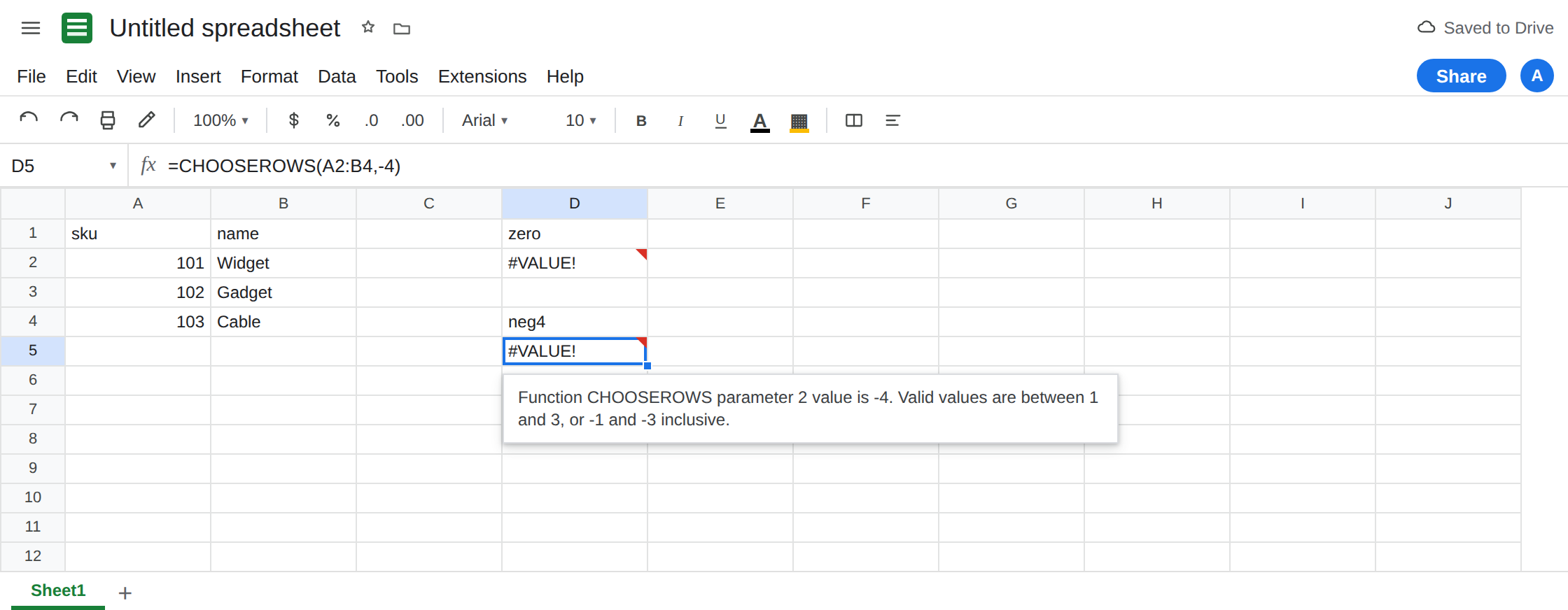
A negative that is too far. In D4 type neg4. In D5 enter =CHOOSEROWS(A2:B4,-4). Three rows. -1, -2, and -3 are the only negative indexes. -4 asks for a row before the start. Same style of tooltip, with -4 in the sentence. Leave D5 broken.

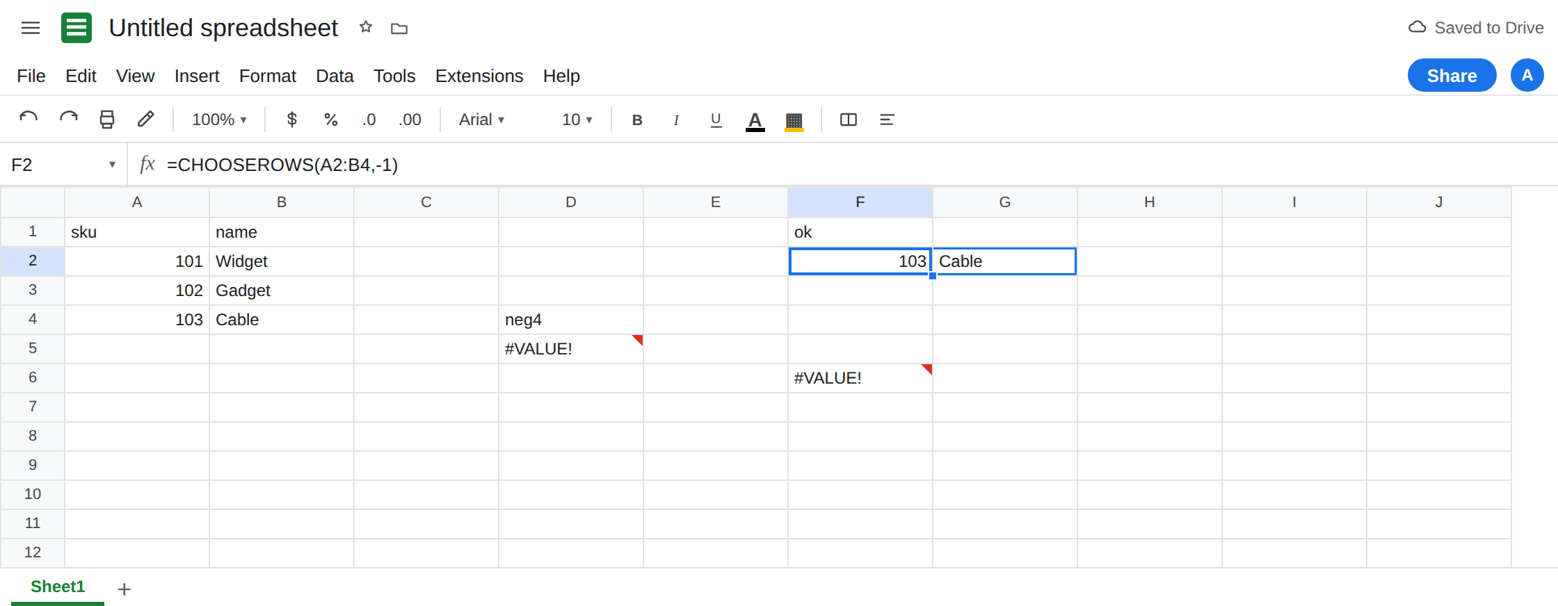
The negatives that work. In F1 type ok. In F2 enter =CHOOSEROWS(A2:B4,-1). The spill is 103 / Cable. In F4 enter =CHOOSEROWS(A2:B4,-3). The spill is 101 / Widget. -3 is the first row, the same row as index 1. Those two spills are the control.

One bad index spoils the list. In F6 enter =CHOOSEROWS(A2:B4,1,-4). You asked for Widget and then for a row that does not exist. The cell errors. You do not get Widget with a blank second row. Leave F6 broken. In F8 enter =CHOOSEROWS(A2:B4,1,3). The spill is Widget and Cable. A list of legal indexes works, including a mix of positive and negative when both exist: =CHOOSEROWS(A2:B4,1,-1) returns Widget and Cable.

Truncation into 0. In D7 enter =CHOOSEROWS(A2:B4,0.9). A non-integer index is truncated toward zero before the range check. 0.9 becomes 0, which is the same error as D2. Leave D7 broken. In D9 enter =CHOOSEROWS(A2:B4,2.9). 2.9 becomes 2. The spill is Gadget. Truncation is not rounding to the nearest row. 2.9 does not become Cable.

Index stored in a cell. In H1 type pick. H2 0. In H4 enter =CHOOSEROWS(A2:B4,H2). H4 errors because H2 is 0, not because the function refuses cell references. Change H2 to -1 and H4 becomes Cable. Put H2 back to 0 and leave H4 broken.

Leave D2, D5, D7, and F6 broken. Leave F2 as Cable.

What is actually wrong

• The legal set on a three-row range is 1, 2, 3, -1, -2, -3. Anything else in that argument is out of range. 0 is the value people use for “no row” or “header.” It is not on the list.
• -1 counts from the bottom of the range, not from the bottom of the sheet. Adding a row under Cable changes what -1 returns. A formula that meant “always Cable” should name row 3 only while the block stays three rows tall, or it should use a key. See VLOOKUP no match if you meant a sku.
• Lists are all-or-nothing. 1,-4 does not mean “row 1, ignore the mistake.” CHOOSEROWS either returns every requested row or errors. A SEQUENCE that runs one step too far (SEQUENCE(4) on a three-row range) fails the same way.
• 0.9 is not “almost the first row.” Truncation toward zero lands on 0 first, and 0 is illegal. 1.1 truncates to 1 and returns Widget. The safe integers are the ones you can count on the range.
• CHOOSECOLS uses the same rules on width. CHOOSECOLS(A2:B4,-3) is out of range because the block is only two columns wide. -1 is the name column. The row primer’s column twin is CHOOSEROWS / CHOOSECOLS.

This is not INDEX #REF!. =INDEX(A2:B4,0,1) is its own error. See INDEX past range. This is not CHOOSE of a value list. See CHOOSE #VALUE!.

Fix

Leave D2, D5, and F6 broken.

Use a negative that fits, or the positive twin. Keep F2: =CHOOSEROWS(A2:B4,-1) for the last row. The first row is 1 or -3 on this block, not 0 and not -4.

Drop the bad index from the list. =CHOOSEROWS(A2:B4,1,3) returns Widget and Cable. If the indexes come from cells, reject 0 before you call: =IF(OR(H2=0,ABS(H2)>ROWS(A2:B4)),"",CHOOSEROWS(A2:B4,H2)). ROWS is 3 here. That guard also blocks -4. Do not wrap D5 in IFERROR. You would hide a picker that asked for a row you do not have. See IFERROR vs IFNA.

Need the header too? Include it in the range. =CHOOSEROWS(A1:B4,-1) is Cable, and relative -1 is now the last of four rows. 0 is still illegal on the taller range.

If the tooltip lists 1 through n and -1 through -n, the index is outside that set. 0, 0.9, and -4 on a three-row block are all outside it. A second index does not rescue the first.