Fix COUNTIFS / SUMIFS #VALUE! in Google Sheets (mismatched range sizes)

COUNTIFS and SUMIFS need every range to be the same size. A criteria range that is taller or shorter than the count or sum range is #VALUE!. The tooltip is Array arguments to COUNTIFS are of different size (or SUMIFS). Same-size ranges that start on different rows do not error. They pair by position and can return 0.

This page is range length. It is not FILTER no match (FILTER mismatch is #N/A), not wrong type (10 + pcs), and not QUERY parse string (Unable to parse query string).

Recreate it on a blank sheet

1. Open a blank spreadsheet. In A1 type sku, B1 region, C1 qty.
2. In A2 type 101. B2 East. C2 10. A3 102. B3 West. C3 20. A4 101. B4 East. C4 5.

COUNTIFS — different heights. In E1 type countifs. In E2 enter =COUNTIFS(A2:A4,101,B2:B5,"East"). A2:A4 is three rows. B2:B5 is four. The cell shows #VALUE!. The tooltip is Array arguments to COUNTIFS are of different size.

E2 selected. Formula bar shows =COUNTIFS(A2,101,B2,"East"). E2 is #VALUE!. Tooltip: Array arguments to COUNTIFS are of different size. A2 is three rows. B2 is four.

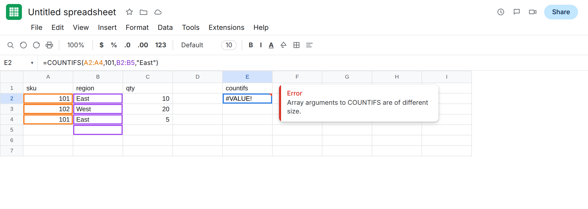
Leave E2 as the broken formula.

SUMIFS — different heights. In G1 type sumifs. In G2 enter =SUMIFS(C2:C4,A2:A4,101,B2:B5,"East"). Sum range C2:C4 is three rows. The second criteria range is four. The cell shows #VALUE!. The tooltip is Array arguments to SUMIFS are of different size.

G2 selected. Formula bar shows =SUMIFS(C2,A2,101,B2,"East"). G2 is #VALUE!. Tooltip: Array arguments to SUMIFS are of different size. E2 is still #VALUE!.

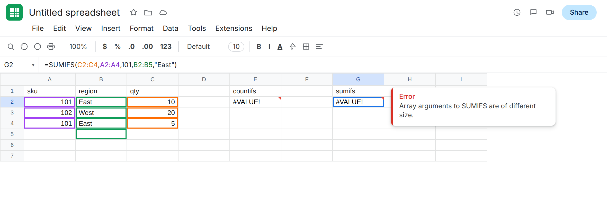
Leave G2 as the broken formula.

Open column vs a bounded range. In E4 type open. In E5 enter =COUNTIFS(A2:A,101,B2:B4,"East"). A2:A runs to the bottom of the sheet. B2:B4 is three rows. The cell shows #VALUE!. Same tooltip.

Leave E5 as the broken formula.

Quiet 0 — same height, shifted rows. In I1 type zeros. In I2 enter =COUNTIFS(A2:A4,101,B3:B5,"East"). Both ranges are three rows. There is no red error. The cell shows 0. Sheets pairs by position: A2 with B3, A3 with B4, A4 with B5. None of those pairs is sku 101 and region East.

Leave I2 as the broken formula.

What is actually wrong

• COUNTIFS and SUMIFS walk the ranges in lockstep. Every criteria range, and the SUMIFS sum range, must have the same number of rows and the same number of columns. Three rows next to four rows is a size error. That is #VALUE!.
• An open-ended column (A2:A or B:B) is not the same height as B2:B4. Mixing them is the same #VALUE!.
• Same height is not enough if the windows are shifted. A2:A4 and B3:B5 are both three cells. They still line up the wrong rows. The formula returns 0 (or a total that ignores the row you can see). There is no tooltip.
• SUMIFS puts the sum range first. COUNTIFS has no sum range — only criteria pairs. Swapping SUMIF argument order into SUMIFS is a different silent 0 (you may be summing a text column). This page is length. Fix the ranges first.

This is not FILTER mismatched range sizes. =FILTER(A2:B4,A2:A5=101) is #N/A. The tooltip names FILTER and the expected row count. See FILTER no match.

This is not #VALUE! from a wrong type. 10 + pcs is Function ADD parameter 2 expects number values. See wrong type. E2 parsed. Then COUNTIFS refused the shapes.

This is not QUERY Unable to parse query string. That #VALUE! is quotes, date 'yyyy-mm-dd', or Col1 vs A inside the query. See QUERY parse string.

This is not a COUNTIF / SUMIF miss on a sku that looks like 101. CHAR(160) returns 1 instead of 2 with no #VALUE!. See CHAR(160) blanks. COUNTIF and SUMIF (one criterion) do not throw this size error the same way. This page is the IFS forms.

Fix

Leave E2, G2, E5, and I2 broken so the size error and the quiet 0 stay on the sheet.

Make every range the same size. Same start row. Same end row. In F1 type countifs_ok. In F2 enter =COUNTIFS(A2:A4,101,B2:B4,"East"). The cell shows 2 (A2 and A4). In H1 type sumifs_ok. In H2 enter =SUMIFS(C2:C4,A2:A4,101,B2:B4,"East"). The cell shows 15 (10 + 5).

F2 selected. Formula bar shows =COUNTIFS(A2,101,B2,"East"). F2 is 2. H2 is 15. I2 is 0. E2, G2, and E5 are still #VALUE!.

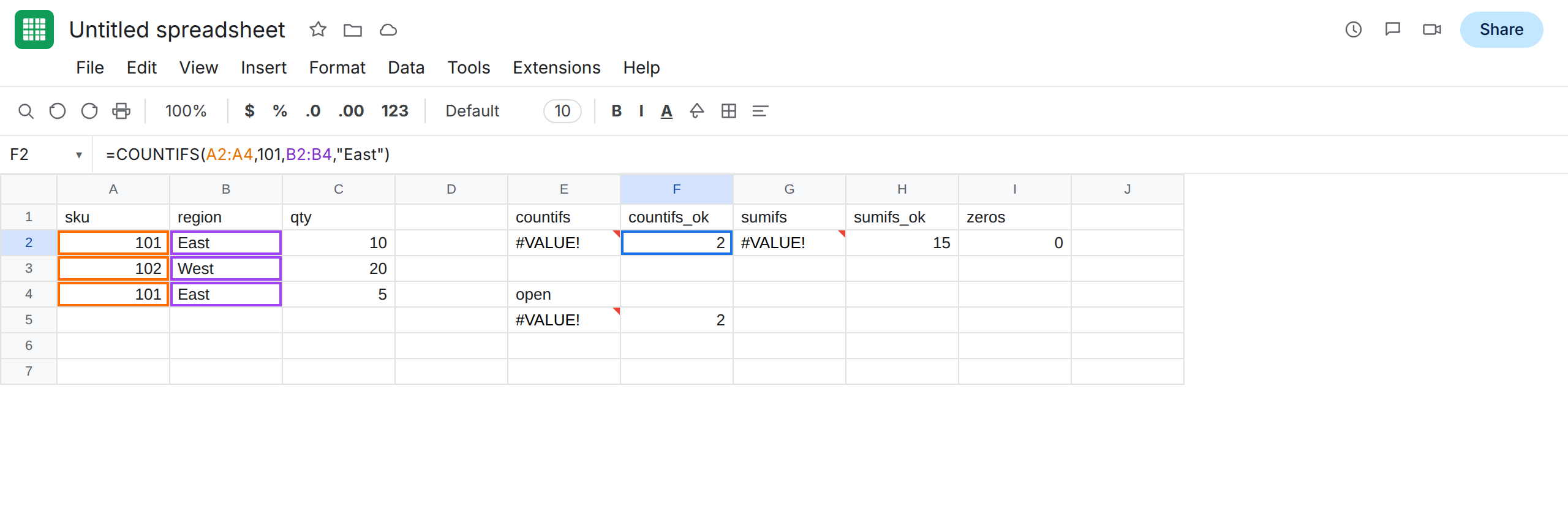
Open columns: open all of them, or none. If the table should grow, use A2:A with B2:B (and C2:C for SUMIFS), not A2:A next to B2:B4. In F5 enter =COUNTIFS(A2:A,101,B2:B,"East"). The cell shows 2. Do not mix a trailing A with a closed B2:B4.

Shifted windows: line up the rows. I2 is 0 because B3:B5 does not sit on the same rows as A2:A4. Point every range at the table: A2:A4 with B2:B4, not B3:B5. F2 already does that.

Do not wrap E2 in IFERROR and call the count fixed. That prints a blank and leaves the ranges different lengths. See IFERROR vs IFNA.

Do not switch this formula to FILTER to “make the sizes match.” A FILTER height mismatch is a different error value. Do not change File > Settings locale. Do not rewrite it as QUERY to dodge the tooltip.

If the tooltip is Array arguments to COUNTIFS are of different size, count the rows in each range in the formula bar. Make them the same. If the cell is 0 and you expected 2, check whether one range starts a row lower than the others.