

Array literal { } parse error in Google Sheets (comma vs backslash, locale)
Updated
{A2,B2} that worked on a US sheet is #ERROR! after File > Settings > Locale. The tooltip says Formula parse error. The braces are fine. The comma inside them is not.
This page is the separators inside { }. Function arguments (VLOOKUP commas vs semicolons) are locale parse error. Do not apply that fix inside an array literal.
Recreate it on a blank sheet
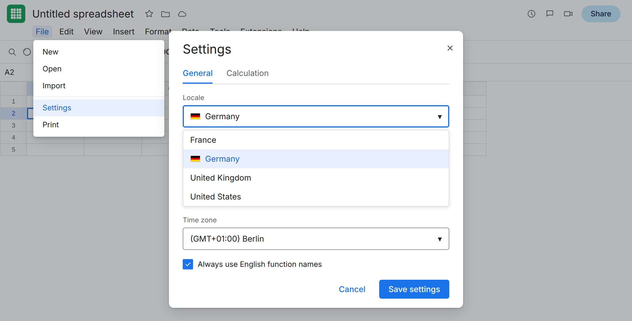
Section titled “Recreate it on a blank sheet”- Open a new blank spreadsheet. File > Settings > Locale → Germany (or Deutsch / Germany). Reload the spreadsheet so the locale actually applies.
- In A2 type
101. B2Widget. - In D2 paste exactly
={A2,B2}with a comma inside the braces. The cell shows#ERROR!. The tooltip is Formula parse error.
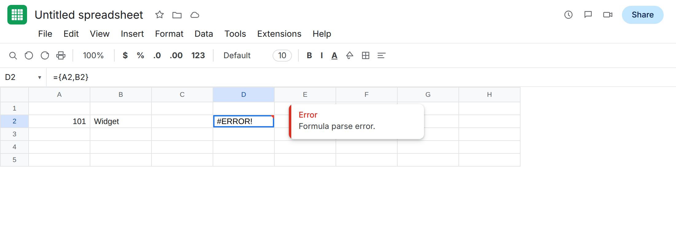
Leave D2 as the broken formula.
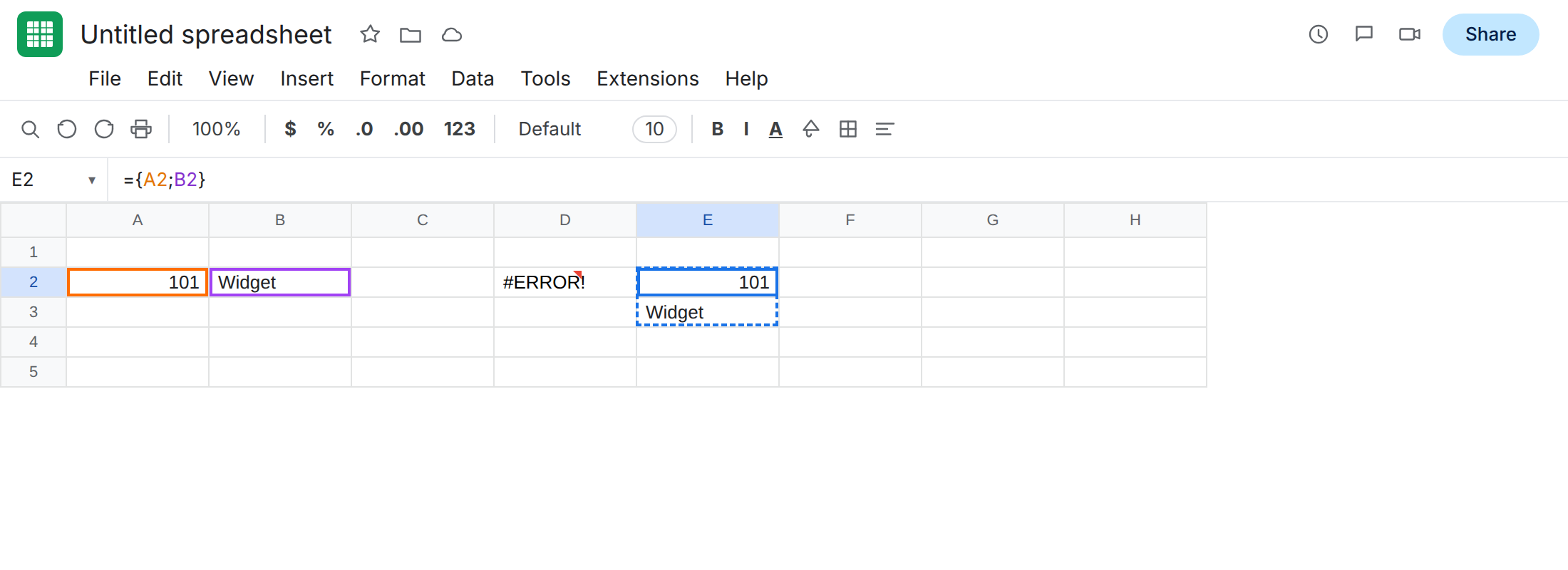
Wrong semicolon. In E2 enter ={A2;B2} with a semicolon. The cell spills 101 then Widget down a column. That parsed. It is not the same shape as {A2,B2} on a US sheet (two columns, one row).
What is actually wrong
Section titled “What is actually wrong”- Inside
{ }, the column separator follows this spreadsheet’s locale. US and UK use a comma between columns. Locales that use a comma as the decimal mark (Germany, France, Brazil) use a backslash (\) between columns. - The row separator is a semicolon in both groups:
{A2;A3}stacks two rows. That is why E2 parsed and D2 did not. - Changing locale does not rewrite formulas.
{A2,B2}copied from a US tutorial, or left over after you switched this file to Germany, is still a comma. Sheets now reads that comma as a decimal mark. Parse error. - Replacing the comma with a semicolon copies the VLOOKUP argument fix. Inside braces that changes columns into rows.
This is not ARRAYFORMULA printing 0 on empty rows. See empty-row zeros. The formula here never ran.
This is not an array that would overwrite a cell. That is #REF!. See SORT / UNIQUE spill.
Leave D2 as the broken formula so the parse error stays on the sheet.
In F2 enter ={A2\B2} with a backslash between the two cells. The spill is 101 in F2 and Widget in G2 — one row, two columns.
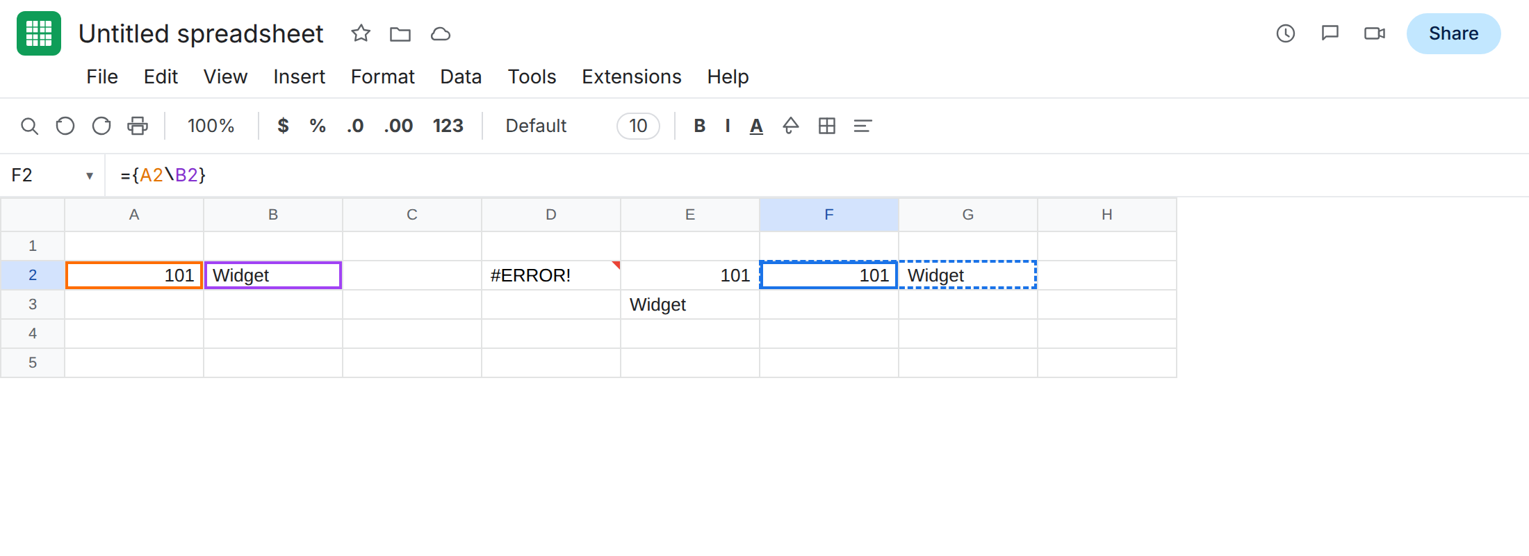
A 2×2 uses both separators. On this German sheet: ={1\2;3\4}. On a US sheet that same grid is ={1,2;3,4}.
Do not change your Google account language. Do not wrap D2 in IFERROR. The only settings change for the recreate is this spreadsheet: File > Settings > Locale, then reload. For a sheet you will keep, type the separators this locale expects.