ERROR.TYPE turns each error into a number you can filter

ERROR.TYPE(reference) returns a number for the error in that cell. The number is stable: #DIV/0! is 2, #VALUE! is 3, #REF! is 4, #NAME? is 5, #NUM! is 6, #N/A is 7. Other errors, including #ERROR!, are 8. #NULL! is 1. If the cell is a normal value, ERROR.TYPE returns #N/A, because there is no error type to report. That #N/A is the function’s own result. It does not mean the cell you tested failed.

ISERROR cannot tell these apart. Both #DIV/0! and #N/A are TRUE. The flags are ISERROR vs ISNA. Wrappers that replace the error are IFERROR vs IFNA. Keep the Google Sheets UI in English. Sheet Error is an independent formula-error library, not a Google product.

Recreate it on a blank sheet

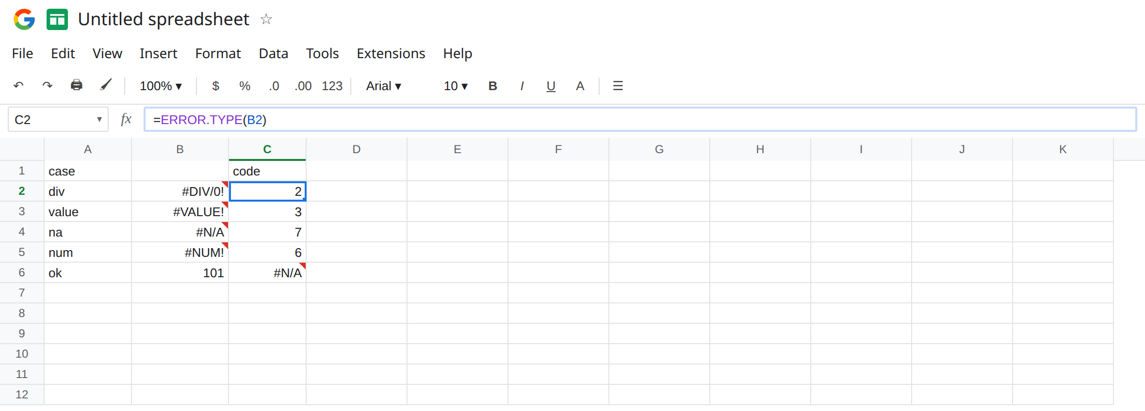
1. Open a blank spreadsheet. In A1 type case. In A2 type div. In A3 type value. In A4 type na. In A5 type num. In A6 type ok.

Build one of each. In B2 enter =1/0. B2 is #DIV/0!. In B3 enter =10+"pcs". B3 is #VALUE!. In B4 enter =NA(). B4 is #N/A. In B5 enter =SQRT(-1). B5 is #NUM!. In B6 type 101. B6 is a number. Leave B2:B5 as errors.

Map them. In C1 type code. In C2 enter =ERROR.TYPE(B2). C2 is 2. In C3 enter =ERROR.TYPE(B3). C3 is 3. In C4 enter =ERROR.TYPE(B4). C4 is 7. In C5 enter =ERROR.TYPE(B5). C5 is 6. In C6 enter =ERROR.TYPE(B6). C6 is #N/A. B6 is fine. ERROR.TYPE returns #N/A when its input is not an error. Leave C6 as that #N/A.

A #REF! so code 4 is on the sheet. In B8 enter =INDEX(A2:A6,9). Row 9 is past a five-row range. B8 is #REF!. In C8 enter =ERROR.TYPE(B8). C8 is 4. See INDEX past range for that #REF!. Do not clear B8.

Filter the codes. In E1 type only_na. In E2 enter =FILTER(A2:B5,C2:C5=7). The spill is the na row: the label and #N/A. Rows whose code is not 7 drop out. FILTER of codes is why the numbers exist. A TRUE/FALSE from ISERROR cannot split #NUM! from #N/A in one pass.

The trap on the good row. In E6 enter =FILTER(A2:A6,C2:C6=7). C6 is itself #N/A. A condition range that contains #N/A does not quietly mean FALSE. Depending on the row, FILTER can return #N/A because the condition failed as an error, not because code 7 was missing. Leave E6 if it errors. The working filter is E2, which stops at C5 and never includes the “no error” #N/A.

Leave C6 as #N/A on a healthy 101. Leave C2 as 2.

What is actually wrong

• The codes are fixed by the product, not by your locale. #DIV/0! is always 2. #N/A is always 7. You can write =IF(ERROR.TYPE(B2)=2,"divisor",B2) and the branch is the divisor case, not “some error.”
• ERROR.TYPE of a normal value is #N/A (code 7’s lookalike). If you copy C2 down through C6, the last cell looks like a lookup miss. It is the “no error” result. ISNA(C6) is TRUE. ISERROR(B6) is FALSE. Test the original cell when you need to know whether anything failed.
• Code 8 is the bucket for errors that are not in the 1–7 list. A formula parse error that still lands in a cell as #ERROR! is that bucket. Do not invent a ninth code.
• IF(ERROR.TYPE(B6)=7,"missing",B6) does not return 101. ERROR.TYPE(B6) is #N/A, and IF cannot compare #N/A to 7. The comparison is #N/A, and IF returns #N/A. Guard with IFNA or test ISERROR first: =IF(ISERROR(B6),ERROR.TYPE(B6),0).
• Filtering C2:C6=7 mixes “this cell is #N/A” with “this cell is not an error.” Stop the condition above the healthy row, or replace C6 with =IFERROR(ERROR.TYPE(B6),0) so a healthy cell is 0 and only real #N/A stays 7.

This is not ISERROR, which collapses every code to TRUE. See ISERROR vs ISNA.

This is not IFERROR(B2,0), which throws the code away and prints 0 for a divisor, a miss, and a bad index alike. See IFERROR hides cause.

Fix

Leave B2:B5 and C6 broken or flagged so the map stays visible.

Read the code, then branch. Keep C2 as =ERROR.TYPE(B2). In G2 enter =IF(ISERROR(B2),ERROR.TYPE(B2),0). G2 is 2. Copy G2 down through G6. G6 is 0, not #N/A. In G8 the same pattern on B8 is 4.

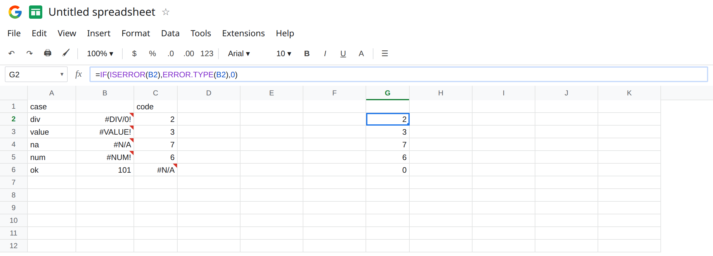
Filter codes 7 only after the guard. =FILTER(A2:B6,G2:G6=7) returns the NA() row and does not treat 101 as a miss.

Use the number in a label, not as a replacement for the fix. Code 2 means go to divide by zero. Code 6 means out of domain or a more specific #NUM! page. The code does not repair the formula.

Do not wrap C6 in IFERROR and call 101 an error that you hid. C6’s #N/A means “no error type.” The repair is the ISERROR guard in G2.

If ERROR.TYPE is #N/A, look at the input. A normal value produces that #N/A. A real #N/A in the input produces 7, not another #N/A. If the number is 2, the input is #DIV/0!. If you filtered on =7 and a healthy row appeared, the condition included an unguarded ERROR.TYPE of a normal cell.

Codes

Code	Error
1	#NULL!
2	#DIV/0!
3	#VALUE!
4	#REF!
5	#NAME?
6	#NUM!
7	#N/A
8	other errors, including #ERROR!

No error in the input is not code 0. It is #N/A from ERROR.TYPE itself, until you guard it.