

Charts gap or drop to zero where the series has #N/A, #DIV/0!, or #VALUE!
Updated
A line chart plots numbers. #N/A, #DIV/0!, and #VALUE! are not numbers. Google Sheets leaves a gap where that point should be. The line does not drop to the axis unless you replace the error with 0. That zero looks like a real month with no units. It is the formula you added, not the chart “breaking.”
SPARKLINE with a bad chart type is SPARKLINE charttype. An empty sparkline range is SPARKLINE empty / args. Divide by zero itself is divide by zero. Keep the Google Sheets UI in English.
Recreate it on a blank sheet
Section titled “Recreate it on a blank sheet”- Open a blank spreadsheet. In A1 type
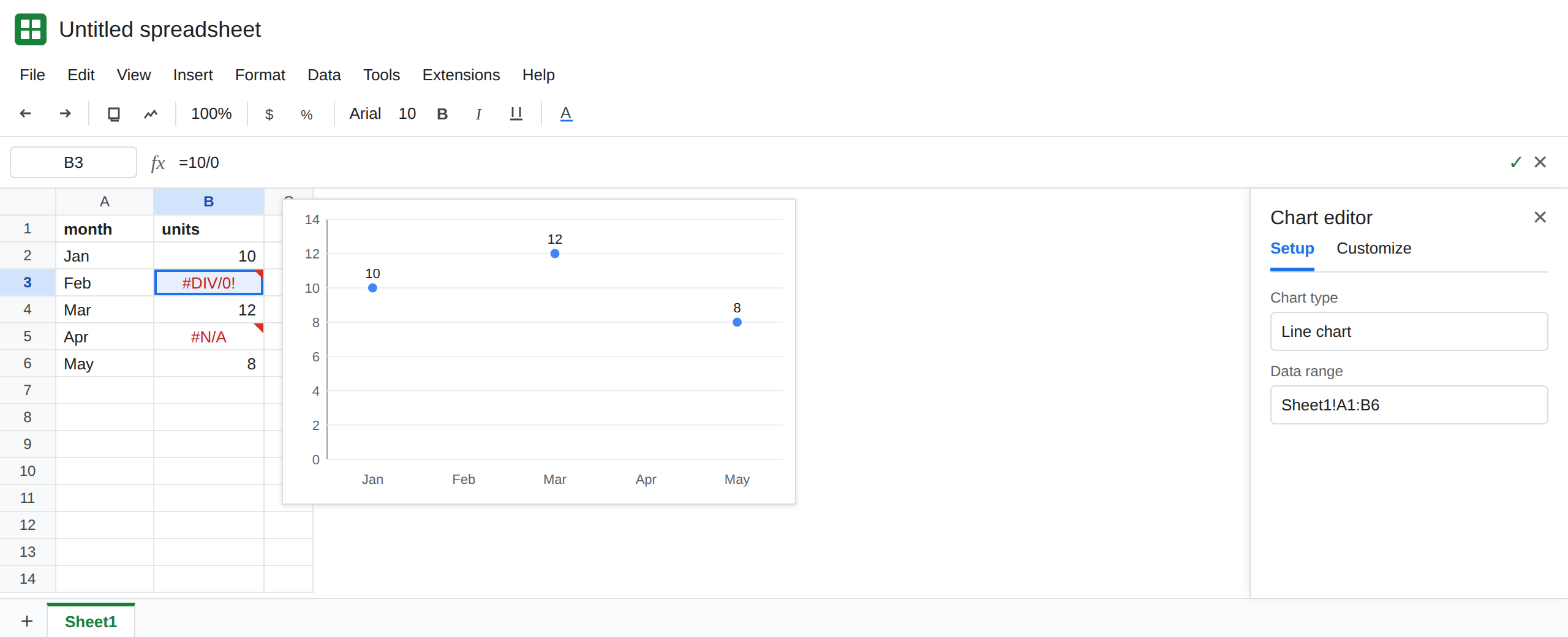
month, B1units. A2Jan, B210. A3Feb. In B3 enter=10/0. B3 is#DIV/0!. A4Mar, B412. A5Apr. In B5 enter=NA(). B5 is#N/A. A6May, B68.
Chart the errors. Select A1:B6. Insert → Chart. In the Chart editor, set the chart type to Line chart if it is not already. The line connects Jan 10, Mar 12, and May 8. February and April are gaps. There is no point on the axis at zero for those two months. The chart is not failing to load. It is skipping cells that are not numbers. Leave B3 and B5 broken.
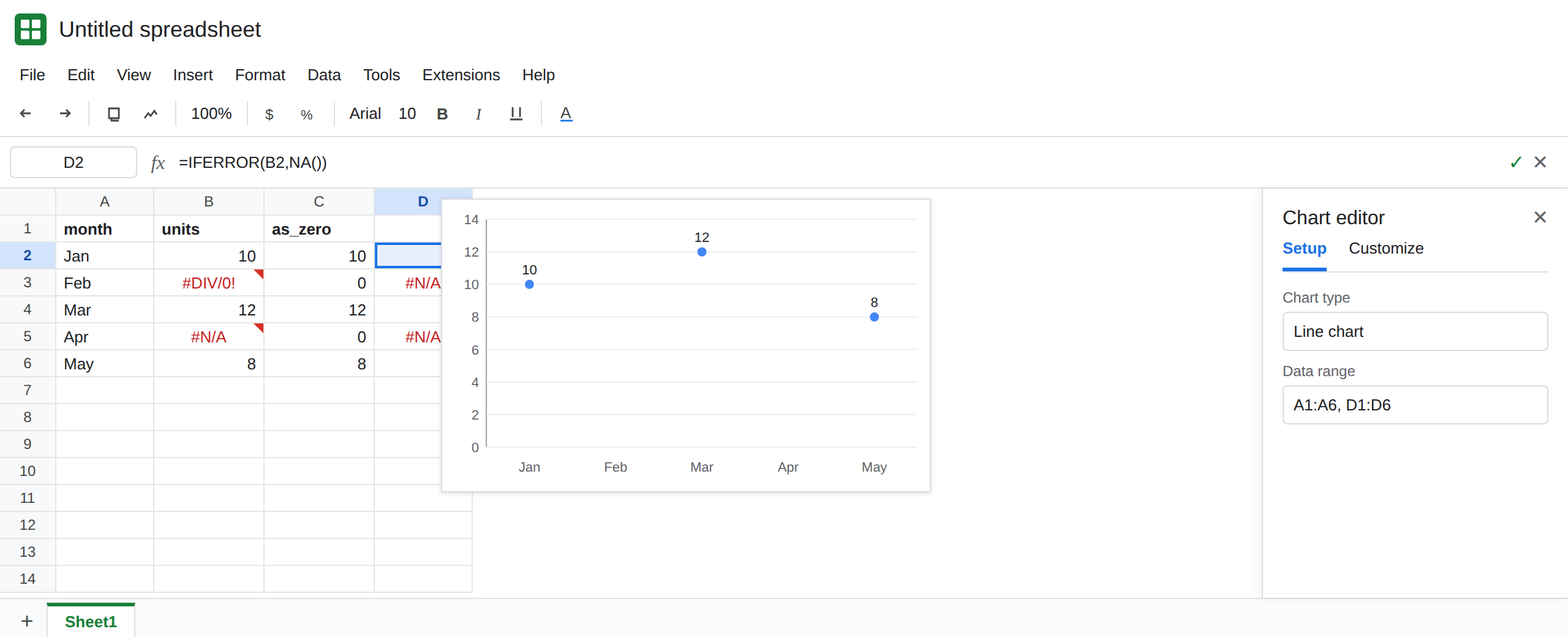
Zero fills the gap. In C1 type as_zero. In C2 enter =IFERROR(B2,0) and fill C2:C6. C3 is 0 because #DIV/0! was replaced. C5 is 0 because #N/A was replaced. C2, C4, and C6 match the real units. Select A1:A6 and C1:C6 and insert a second line chart (or change the first chart’s data range to include column C and not B). The line touches the axis in February and April. Those zeros are not in the source. IFERROR wrote them.
A blank is closer to a gap than a zero is. In D2 enter =IFERROR(B2,NA()) and fill D2:D6. D3 and D5 are #N/A. A line chart of column D gaps there, the way column B does. NA() is a gap you chose. 0 is a point you chose.
#VALUE! skips the same way. In B6, temporarily type pcs over the 8 only if you want to see #VALUE! from a later formula. For this sheet, leave B6 as 8. A text cell in the series is not plotted as a number either. Do not format the error cells as Number and expect the triangle to become a zero. Format does not change #DIV/0!.
What is actually wrong
Section titled “What is actually wrong”- The chart series is numeric.
#DIV/0!means the formula divided by zero. See divide by zero.#N/Ameans not available. See what #N/A means.#VALUE!means the wrong type. See wrong type. None of those is the number 0. - Google Sheets does not plot those errors as zero. The line breaks (a gap) or the point is absent. That is the chart telling you the cell is not a value.
IFERROR(B3,0)runs before the chart does. The chart then honestly plots 0. The misleading part is the formula, not Insert → Chart.IFERRORalso turns#N/Ainto 0. A missing April and a broken February become the same point.IFNAonly replaces#N/A. See IFERROR vs IFNA.- Excel’s chart dialog is Select Data → Hidden and Empty Cells. The choices are gaps, zero, or connect data points with a line, plus a checkbox to show
#N/Aas an empty cell. That dialog is Excel. It is not a Sheets Chart editor tab. Do not look for those exact words in Google’s Customize panel. In Sheets, change the cells the series reads.
This is not a sparkline charttype typo. A sheet chart uses the Chart editor. SPARKLINE is a formula.
Leave B3 as #DIV/0! and B5 as #N/A. Leave the first chart gapped so the errors stay visible.
Repair the cell when the month should have a number. February divided by zero is a source bug. Fix the divisor. Do not paint 0 over it for the picture. When B3 becomes a real units figure, the line picks the point up. No chart setting required.
Keep a gap when the month is missing. Leave #N/A, or write =NA(), in that row. Chart column B or column D. The gap is the honest mark. Use =IFNA(B5,NA()) only when you are already holding a miss and you want it to stay a miss. Use IFERROR to 0 only when zero units is the true value.
In Excel, open Select Data → Hidden and Empty Cells if you want gaps versus zeros for empty cells, and turn on show #N/A as an empty cell when a missing point must not become zero. Still fix a real #DIV/0! in the grid. The dialog does not repair the formula.
If the line touches zero only after an IFERROR to 0, the chart is plotting that zero. If the line gaps on #N/A and #DIV/0!, the chart is skipping errors. Put a real number in the cell when you want a point.