N() turns text into 0, so a SUMPRODUCT check still looks valid

N(value) returns a number. A number stays that number. TRUE becomes 1. FALSE becomes 0. A date becomes its serial. Text becomes 0. There is no #VALUE! and no warning. N("abc") is 0, the same result as N(FALSE) and the same result as a real 0 you typed. A SUMPRODUCT that wraps a column in N will add that zero and look finished. The word in the cell never had a chance to break the total.

Coercing TRUE and FALSE with *1 or -- is SUMPRODUCT booleans. A #VALUE! because two arrays have different shapes is SUMPRODUCT size. Keep the Google Sheets UI in English. Sheet Error is an independent formula-error library, not a Google product.

Recreate it on a blank sheet

1. Open a blank spreadsheet. In A1 type flag. These are supposed to be 1 for yes and 0 for no.

In A2 type 1. A3 type 1. A4 type abc. A5 type 0. Three numeric flags and one word. The two yes flags should total 2 if the word is thrown out. They also total 2 if the word is treated as no. Those are not the same audit.

N on the word. In C1 type n_word. In C2 enter =N(A4). C2 is 0. No error triangle. In C3 enter =ISTEXT(A4). C3 is TRUE. The source is text. N reported a number anyway. In C4 enter =N(TRUE). C4 is 1. In C5 enter =N(FALSE). C5 is 0. C2 and C5 match. A word and a boolean false are the same output.

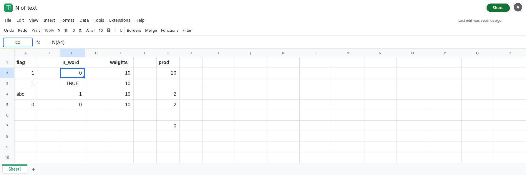
The check that hides it. In E1 type weights. E2 10, E3 10, E4 10, E5 10. In G1 type prod. In G2 enter =SUMPRODUCT(N(A2:A5),E2:E5). G2 is 20. That is 1*10 + 1*10 + 0*10 + 0*10. The abc row contributed the same 0 as the real zero in A5. Nothing in G2 says a label was illegal. Leave G2 as 20.

SUM skips the word and lands on the same 2. In G4 enter =SUM(A2:A5). G4 is 2. SUM ignores text. It does not turn the word into a zero you can see inside the array, but the displayed total matches =SUMPRODUCT(N(A2:A5)), which is also 2. Matching totals are why the sheet looks reviewed. In G5 enter =SUMPRODUCT(N(A2:A5)). G5 is 2.

A header is text too. In G7 enter =N(A1). G7 is 0. flag is not a number. If a total starts at A1, N swallows the header as zero instead of breaking. The numeric flags below still add.

Leave G2 as 20. Leave C2 as 0.

What is actually wrong

• N is a converter with a trash bin. Anything it does not recognize as a number, a boolean, or a date becomes 0. The trash bin is silent. ISTEXT on the source is still TRUE.
• Inside SUMPRODUCT, that 0 is a real term. It multiplies the paired weight and adds nothing. A row you meant to reject looks like a row whose flag was no.
• SUM ignoring text and N converting text to 0 can print the same total on a single column of flags. The difference shows up when the converted 0 is multiplied by another array, or when you later count zeros as answered “no”.
• N of TRUE is 1. That part is useful. Wrapping a mixed column, header included, throws the useful case and the trash bin into one number.
• An error value in the range is not text. Do not wrap N in IFERROR to hide it. See IFERROR vs IFNA. You would lose the triangle and still have a made-up zero if you substitute 0.

This is not the boolean-coercion zero, where every comparison stayed TRUE/FALSE and the product was 0 until you multiplied by 1. See SUMPRODUCT booleans. Here the total is nonzero and one input was a word.

Fix

Leave C2 and G2 in place. G2 is the quiet wrong total. C2 is the proof that the word became 0.

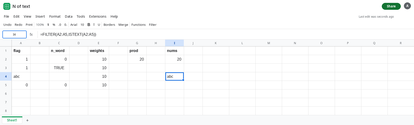
Count only real numbers, and list the text. In I1 type nums. In I2 enter =SUMPRODUCT((ISNUMBER(A2:A5))*(A2:A5),E2:E5). I2 is 20 as well, but the mask is explicit: text fails ISNUMBER and drops out. In I4 enter =FILTER(A2:A5,ISTEXT(A2:A5)). I4 spills abc. That spill is the row G2 treated as a zero flag. If I4 is #N/A, there is no text in the flags and N was not hiding a word. See FILTER no match.

Or reject the column before you multiply. =IF(COUNTIF(A2:A5,"?*")>0,"text in flags",SUMPRODUCT(N(A2:A5),E2:E5)) prints text in flags while A4 is abc. The ?* wildcard matches a text cell with at least one character. A blank flag does not match it. See COUNTIF literal * ? if a flag really contains a star.

Do not replace N with IFERROR. The word was never an error. N already succeeded.

If N of a cell is 0 and ISTEXT of that cell is TRUE, the zero is the converter, not a flag. If every cell in the flag column is ISNUMBER or a boolean, N is doing the coercion you asked for. If the total is 0 and the flags are TRUE/FALSE with no N at all, you are on the boolean page.