VLOOKUP returns the wrong row in Google Sheets (TRUE approximate match)

You look up sku 200 and VLOOKUP hands back Lamp, not Chair. The formula ran. It matched the wrong row. That is not #N/A. Approximate match (TRUE, or a missing fourth argument) walks the first column as if it were sorted ascending. An unsorted sku list still “matches.” It matches the wrong row.

Recreate it on a blank sheet

1. Open a blank spreadsheet. In A1 type sku, B1 name. Leave column C empty. D1 lookup, E1 TRUE, F1 omitted, G1 FALSE.
2. Type the table in this order — 200 first, then 100, then 150. A2 200, B2 Chair. A3 100, B3 Desk. A4 150, B4 Lamp. In D2 type 200.
3. In E2 enter =VLOOKUP(D2,A2:B4,2,TRUE). The cell shows Lamp.

E2 selected. Formula bar shows =VLOOKUP(D2,A2,2,TRUE). E2 is Lamp. Unsorted 200 / 100 / 150 is visible; F2 is Lamp and G2 is Chair.

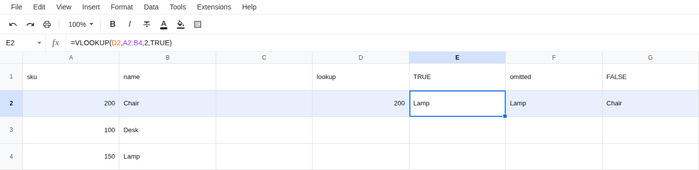
Leave E2 as the broken formula.

4. In F2 enter =VLOOKUP(D2,A2:B4,2) with no fourth argument. That cell is also Lamp. Omitting the fourth argument is the same as TRUE.

Leave F2 broken.

Second recreate — a sku that is not on the table still returns a row. In D4 type 999. In E4 enter =VLOOKUP(D4,A2:B4,2,TRUE). The cell shows Lamp, not #N/A. Approximate match does not require an exact key. It lands on a nearby row in sorted-order logic. On this unsorted list that nearby row is the last one. In F4 enter =VLOOKUP(D4,A2:B4,2,FALSE). The cell shows #N/A. That is the miss you wanted. Leave E4 as Lamp so the two fourth-arguments stay on the sheet.

What is actually wrong

The fourth argument is the match mode. TRUE means approximate match. Leaving it off is the same as TRUE. Approximate match walks the first column as if it were sorted ascending. This list is not: 200, then 100, then 150.

Sku 200 is sitting in A2 next to Chair. Approximate match still returns Lamp from the last row. The function did not fail. It followed TRUE rules on a list that is not sorted. That is why there is no red triangle on E2.

FALSE is exact match. It finds 200 and returns Chair. For 999 it returns #N/A, which is correct when the sku is absent.

This is not a missing key that should have been #N/A on E2. 200 is on the sheet. See what #N/A means for an actual miss. This page is a hit on the wrong row, and a miss that TRUE refuses to call a miss.

This is not number vs text. All skus here are numbers. See VLOOKUP no match. This is not lookup-left. The search column is sku. See lookup left of the key. This is not a column index past the range. Index 2 is legal on A2:B4. See VLOOKUP bad index.

XLOOKUP without a match mode is exact. Migrating and dropping FALSE because “XLOOKUP does not need it” is correct. See XLOOKUP vs VLOOKUP. Keeping a bare VLOOKUP is this bug.

Fix

For sku lookups, always pass FALSE. Leave E2, F2, and E4 as the broken formulas so the wrong row stays on the sheet.

In G2 enter =VLOOKUP(D2,A2:B4,2,FALSE). The cell shows Chair.

G2 selected. Formula bar shows =VLOOKUP(D2,A2,2,FALSE). G2 is Chair. E2 is still Lamp.

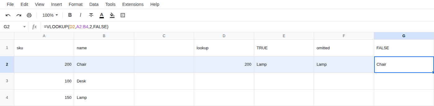
In G4 enter =VLOOKUP(D4,A2:B4,2,FALSE). The cell shows #N/A. Wrap that miss with IFNA only if a missing sku is a valid result. See IFERROR vs IFNA. Do not wrap E2. E2 is not a miss.

Sku lookups are exact. FALSE is the argument that does that. Do not sort the table to make TRUE look right — that is not the fix. Approximate match is for bands (tax brackets, quantity breaks) on a list you keep sorted on purpose. A sku column is not a band.