Fix XLOOKUP #N/A in Google Sheets (no match vs if_not_found)

XLOOKUP returns #N/A when the search key is not in the lookup range. The formula ran. There was no match. That is the same error value as a VLOOKUP miss. It is not a broken function and not a reason to switch match modes until you have confirmed the key is absent.

This page is an exact XLOOKUP miss, and the two ways to replace #N/A with a fallback: the fourth argument (missing_value in Sheets; Excel callers know the same slot as if_not_found) versus wrapping IFNA. It is not VLOOKUP no match (number vs text, or a trailing space). It is not XLOOKUP vs VLOOKUP (left lookup, default exact match, the migration). It is not lookup left of the key.

Recreate it on a blank sheet

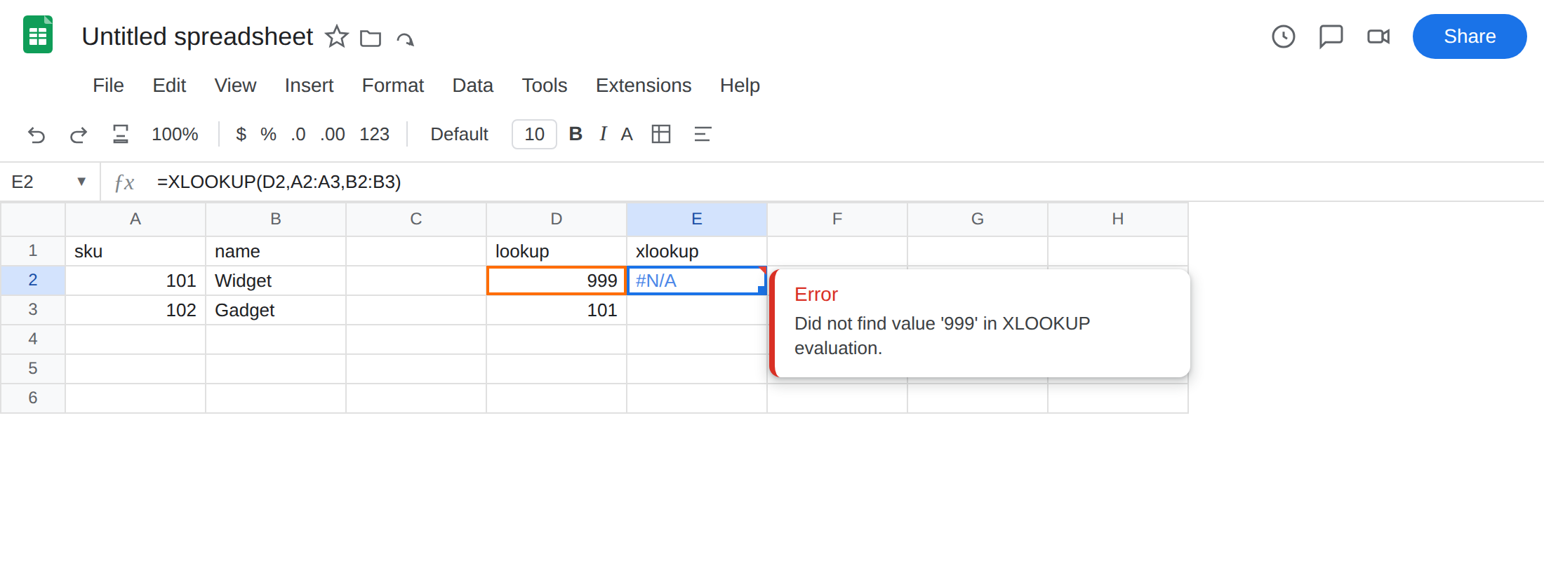
1. Open a blank spreadsheet. In A1 type sku, B1 name. A2 101 as a number. B2 Widget. A3 102. B3 Gadget. D1 lookup. D2 999 — that sku is not in column A. D3 101.
2. Exact miss. In E1 type xlookup. In E2 enter =XLOOKUP(D2,A2:A3,B2:B3). The cell shows #N/A. The tooltip is Did not find value ‘999’ in XLOOKUP evaluation. Leave E2 broken.

3. A hit on the same table. In E3 enter =XLOOKUP(D3,A2:A3,B2:B3). The cell shows Widget. Same function, same ranges. D3 is on the sheet. That row is the control: XLOOKUP works when the key exists.

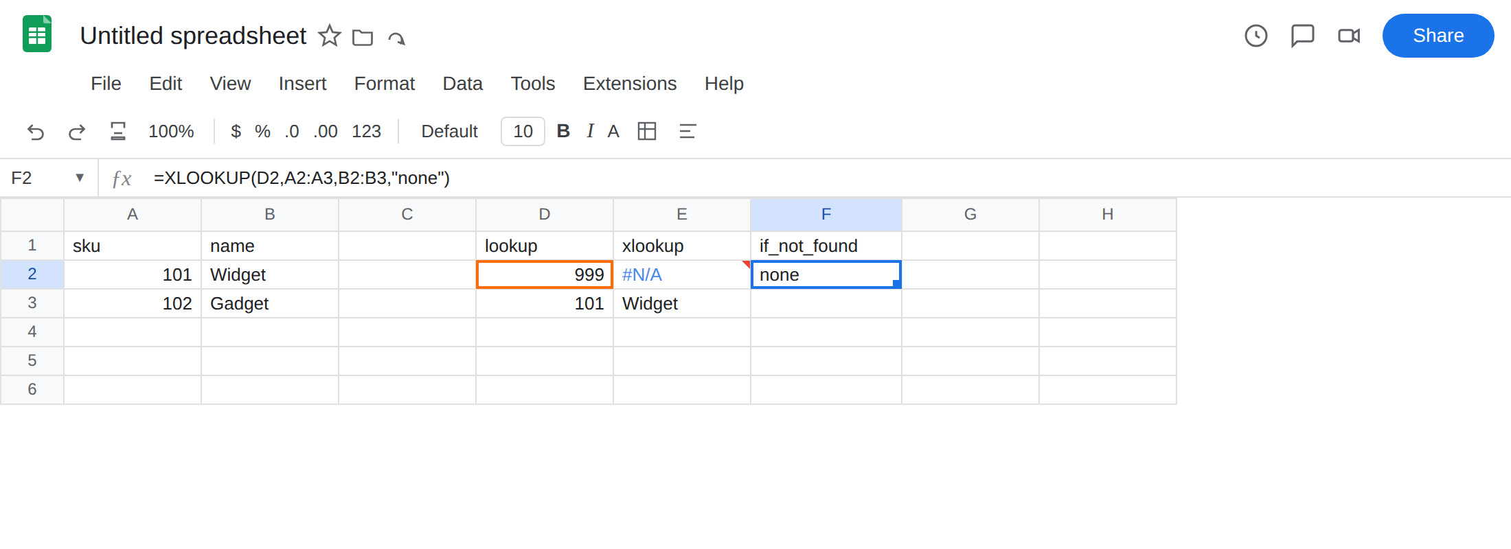
if_not_found on the miss. In F1 type if_not_found. In F2 enter =XLOOKUP(D2,A2:A3,B2:B3,"none"). The cell shows none. The fourth argument fired because 999 is missing. It did not change E3. Leave E2 as the raw #N/A so you can compare.

IFNA around a bare XLOOKUP. In G1 type ifna. In G2 enter =IFNA(XLOOKUP(D2,A2:A3,B2:B3),"none"). The cell shows none. Same fallback as F2. The wrapper sits outside the function. The fourth argument sits inside it.

IFERROR also looks like a miss. In H1 type iferror. In H2 enter =IFERROR(XLOOKUP(D2,A2:A3,B2:B3),"none"). The cell shows none. Then in I1 type bad_range. In I2 enter =XLOOKUP(D2,A2:Z2,B2:B3). Lookup and result ranges are different sizes. I2 errors. In I3 enter =IFERROR(XLOOKUP(D2,A2:Z2,B2:B3),"none"). The cell shows none. In I4 enter =XLOOKUP(D2,A2:Z2,B2:B3,"none"). The fourth argument does not turn a broken range into none. The miss argument is the miss only.

Confirm the miss before you wrap. Type 101 in D2. E2 becomes Widget. Put 999 back so #N/A returns. If changing the lookup value makes #N/A come and go, the function is working and the key is absent.

What is actually wrong

• 999 is not in A2:A3. XLOOKUP defaults to exact match (match_mode 0). No row qualifies. The result is #N/A.
• The fourth argument (missing_value / if_not_found) replaces that #N/A only. A size mismatch, a #REF! range, or #DIV/0! inside a more complex formula still surfaces. That is the same idea as IFNA. See IFERROR vs IFNA. An empty fourth argument is not a blank cell. See XLOOKUP blank fallback.
• IFNA(XLOOKUP(...),"none") and XLOOKUP(...,"none") agree on a miss. They disagree on everything else only when you compare them to IFERROR. IFERROR will also print none for a bad range. F2 will not.
• XLOOKUP does not coerce number vs text. If D2 were text '101 and A2 were numeric 101, E2 would still be #N/A with the sku “on the sheet.” That is VLOOKUP no match, and XLOOKUP fails the same keys until you clean them. if_not_found will not fix type.
• A name that sits left of sku is not this recreate. =XLOOKUP(101,A2:A3,B2:B3) searches sku and returns name. Searching the wrong column is lookup left of the key. The migration page is XLOOKUP vs VLOOKUP.

This is not FILTER with zero rows. See FILTER no match. This is not REGEXEXTRACT. See REGEX no match.

Fix

Leave E2 as the raw #N/A. Leave I2 as the broken range.

When a miss is not allowed. Put the sku on the table, or fix the key. Do not add if_not_found so a missing 999 looks like a real name. E3 already proves the formula works for 101.

When a miss is a valid result. Prefer the fourth argument. Keep F2: =XLOOKUP(D2,A2:A3,B2:B3,"none") returns none. That is if_not_found. You do not need IFNA around a function that already has a miss slot.

If you must wrap. =IFNA(XLOOKUP(D2,A2:A3,B2:B3),"none") matches F2 on this miss. Use it when the XLOOKUP is already written without a fourth argument and you do not want to touch the inner call. Do not upgrade that wrap to IFERROR “to be safe.”

Do not switch to VLOOKUP to clear #N/A. VLOOKUP has no miss argument. Stay on XLOOKUP. Fix the key, or pass if_not_found.

When to use if_not_found instead of IFERROR

Use if_not_found (the fourth argument) when the only thing you want to hide is “this key is not in the list.” A dashboard that should print none for an unknown sku, and should still scream when someone points XLOOKUP at ranges of different heights, is that case.

Use IFERROR only when every error should look the same. That is rare for a lookup column. IFERROR will also swallow a #REF! from a deleted name, a #NAME? from XLOKUP, and a shape error. Those are bugs. They are not misses. if_not_found leaves them visible. So does IFNA. IFERROR does not.

If the sku is on the sheet and XLOOKUP is still #N/A, stop wrapping. Check type and spaces first. Then, if the key is truly absent and a fallback is allowed, pass if_not_found.