

ARRAYFORMULA with IFERROR masks #DIV/0! and #N/A as blank or 0
Updated
ARRAYFORMULA spills one formula down a column. IFERROR around that formula spills too, and it replaces every error with whatever fallback you typed. A #DIV/0! becomes 0 or a blank. A #N/A from VLOOKUP becomes a blank bay. The column has no red triangles. The zeros look like measured rates.
This page is that mask. It is not ARRAYFORMULA AND/OR (those two functions collapse to one boolean). It is not empty-row zeros (a blank cell coerced to 0 in arithmetic). IFERROR versus IFNA as a choice on one cell is IFERROR vs IFNA.
Recreate it on a blank sheet
Section titled “Recreate it on a blank sheet”- Open a blank spreadsheet. Keep the Google Sheets UI in English. In A1 type
units, B1hours. A210, B22. A310, B30. A45, B45. Row 3 divides by zero on purpose.
Unmasked spill. In D1 type raw. In D2 enter =ARRAYFORMULA(A2:A4/B2:B4). D2 shows 5. D3 shows #DIV/0!. D4 shows 1. The tooltip on D3 is the divide-by-zero error. That triangle is the diagnosis. Leave D2:D4 as they are.
Mask to zero. In F1 type mask_0. In F2 enter =ARRAYFORMULA(IFERROR(A2:A4/B2:B4,0)). F2 shows 5. F3 shows 0. F4 shows 1. No triangle on F3. A rate of zero hours-per-unit is a real number in a dashboard. Here it means “B3 was zero and the error was deleted.”
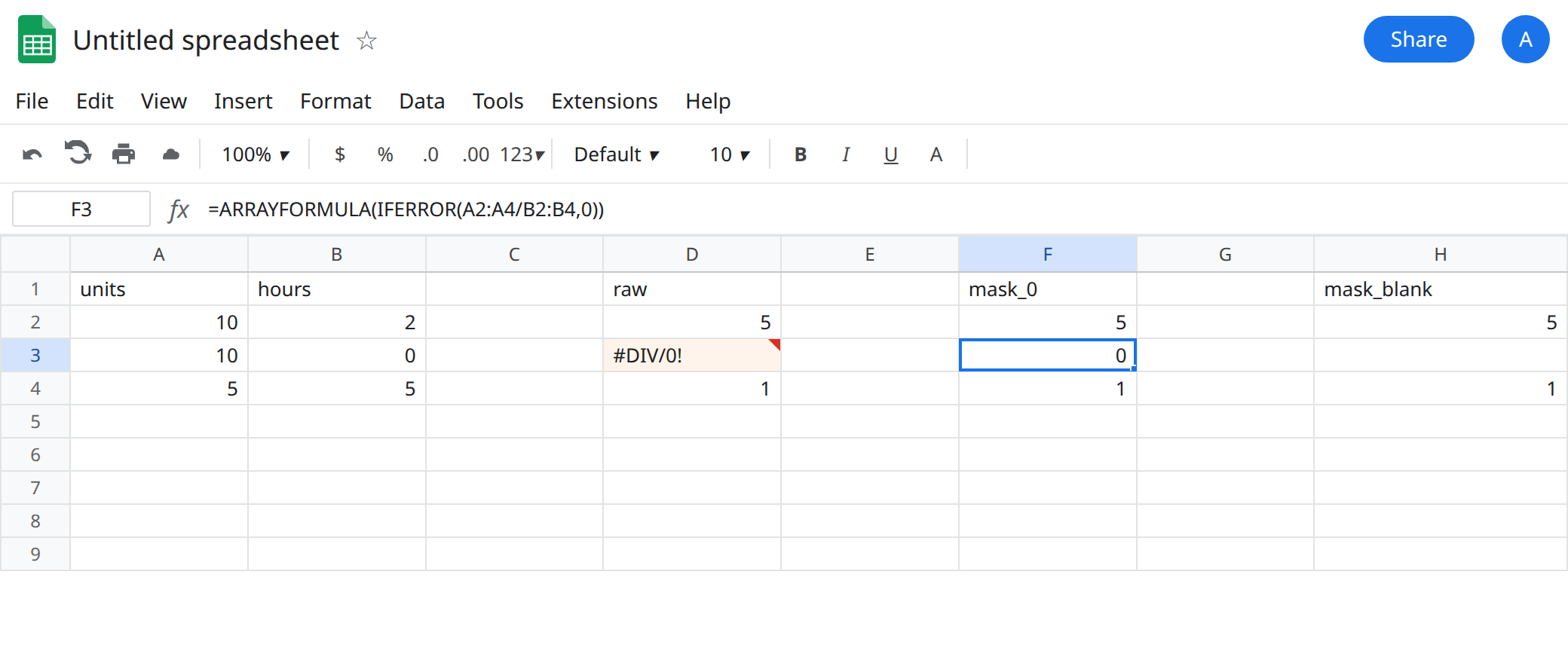
Mask to blank. In H1 type mask_blank. In H2 enter =ARRAYFORMULA(IFERROR(A2:A4/B2:B4,"")). H3 looks empty. =H3="" is TRUE. =ISBLANK(H3) is FALSE, because the spill wrote an empty string. A chart skips the blank and the zero differently. Neither one is #DIV/0!.
Lookup mask. In J1 type sku, K1 bay. J2 101, K2 A. J3 102, K3 B. In M1 type find. M2 101. M3 999. M4 102. In O1 type lookup_mask. In O2 enter =ARRAYFORMULA(IFERROR(VLOOKUP(M2:M4,J2:K3,2,FALSE),"")). O2 is A. O3 looks empty. O4 is B. The unmasked formula =VLOOKUP(M3,J2:K3,2,FALSE) in Q3 is #N/A, tooltip Did not find value ‘999’ in VLOOKUP evaluation. O3 hid that miss. Leave Q3 broken. Leave O3 blank.
=ARRAYFORMULA(IF(ISERROR(A2:A4/B2:B4),"",A2:A4/B2:B4)) is the same mask as H2. ISERROR is true for #DIV/0!, #N/A, #VALUE!, and #REF!. One fallback eats all of them.
What is actually wrong
Section titled “What is actually wrong”IFERROR(value, fallback)returnsfallbackwhenvalueis any error. InsideARRAYFORMULA, that decision runs on every row. F3’s0is the fallback you typed, not10/0.- A blank fallback is still a value. H3 is
"". ISBLANK vs empty is FALSE for that cell.COUNTBLANKwill count it. A pivot that drops blanks drops the row. You did not filter. You erased the error. IFERRORis wider than the bug. F2 also hides#N/A,#VALUE!, and#REF!if a later edit introduces them. You cannot see which one you hit.IFNAwould hide Q3’s miss and would not hide D3’s#DIV/0!. PickingIFERRORbecause “IFNAleft the triangle” is how divide-by-zero becomes zero.- The
IF(ISERROR(...),"", value)form calculates the division twice and still masks every error type. It is not a narrower test. - A guard is different from a mask.
=ARRAYFORMULA(IF(B2:B4=0,"",A2:A4/B2:B4))blanks only the zero divisor. If A3 is text,#VALUE!still shows. That is what you want while you clean the column.IFERRORwould hide the text too. VLOOKUPinside the same wrapper turns a missing sku into an empty bay (O3). The nextCOUNTIFon column O under-counts misses. See VLOOKUP #N/A for the miss itself. Do not fix a miss by deleting it.
This is not AND/OR collapsing a spill. F2 spilled three cells. The values are wrong; the shape is right. Empty cells multiplied in an array can also show 0. That page is empty-row zeros. B3 here is a typed 0, and D3 is #DIV/0!, not a quiet zero.
Leave F2, H2, and O2 on the sheet. They are the bug. Keep D2 and Q3 as the unmasked pair.
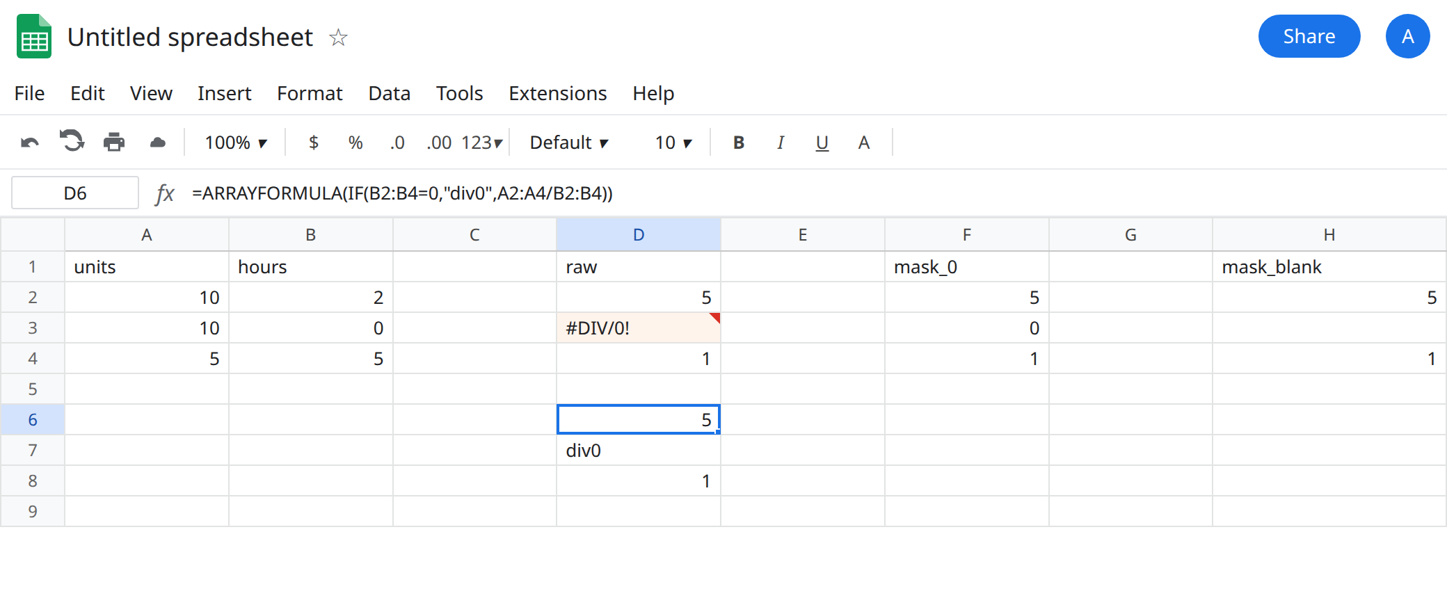
Guard the case you mean. For this hours column, in D6 enter =ARRAYFORMULA(IF(B2:B4=0,"div0",A2:A4/B2:B4)). D7 (the second spill row) shows div0. D6 shows 5. D8 shows 1. The label is visible. A text hours cell would still error.
Lookups: IFNA on purpose, and not inside the only copy. =ARRAYFORMULA(IFNA(VLOOKUP(M2:M4,J2:K3,2,FALSE),"missing")) shows missing for sku 999. Use that only after Q3 has taught you the tooltip. Do not use IFERROR for a lookup. A #REF! from a bad column index would become "missing" too. See IFERROR vs IFNA.
Divide-by-zero as its own page. One cell =A3/B3 is divide by zero. The array does not change the arithmetic. It only copies it.
If a spilled column is all numbers and one of them sits on a zero divisor, open the formula and look for IFERROR or ISERROR. Put the raw ARRAYFORMULA beside it until the triangle is back.