FIND is case-sensitive and SEARCH is not, and only SEARCH treats * and ?

FIND(search_for, text, [start]) and SEARCH(search_for, text, [start]) both return the position where a substring starts. FIND matches case. SEARCH does not. SEARCH also treats ? as one character and * as any run of characters. FIND looks for those marks as letters. On the text Widget Pro, FIND of pro is #VALUE! and SEARCH of pro is 8. The letters are on the sheet. The case, or the wildcard, is what changed.

A needle that is absent in both functions, such as xyz inside Widget, is FIND / SEARCH miss. This page does not rebuild that miss. REGEXMATCH case flags are REGEXMATCH case. Keep the Google Sheets UI in English. Sheet Error is an independent formula-error library, not a Google product.

Recreate it on a blank sheet

1. Open a blank spreadsheet. In A1 type text. In A2 type Widget Pro. Count the characters if you want the positions in front of you: W is 1, the space is 7, P is 8, o is 10. Eleven characters. LEN(A2) is 11.

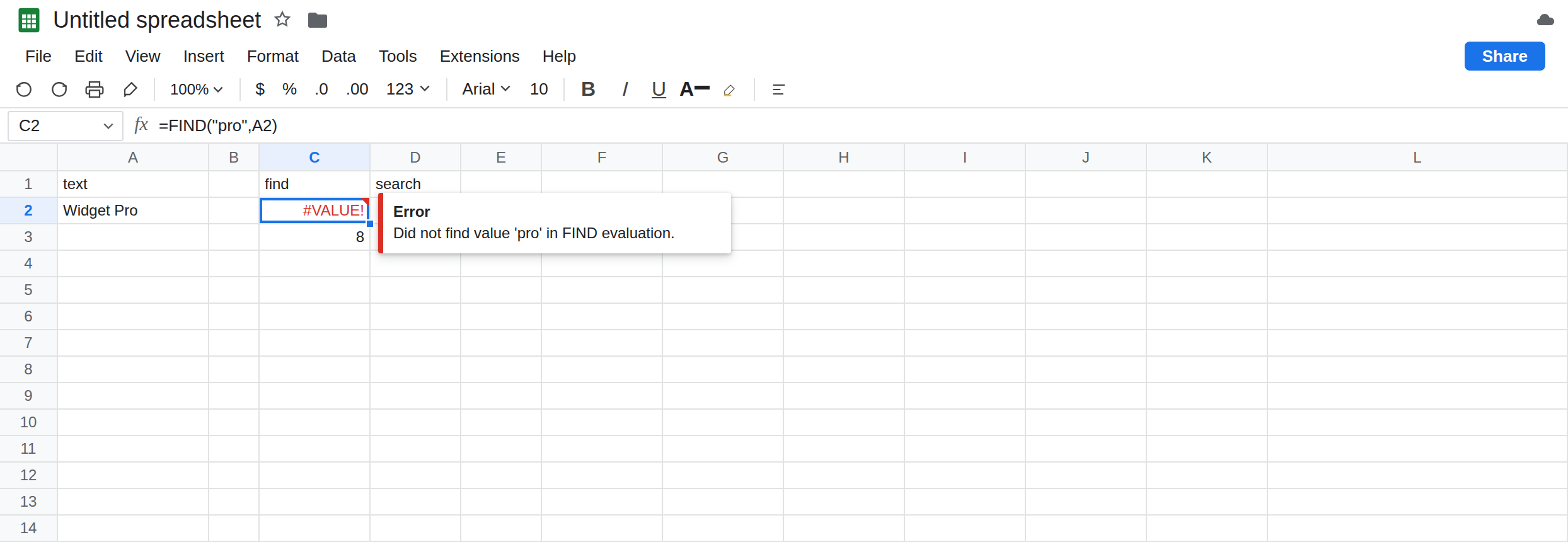
Case. In C1 type find, D1 search. In C2 enter =FIND("pro",A2). C2 is #VALUE!. The tooltip says Sheets did not find pro. The cell Pro is sitting in A2 with a capital P. FIND will not fold it. In D2 enter =SEARCH("pro",A2). D2 is 8. SEARCH ignores case, so pro starts at the P. In C3 enter =FIND("Pro",A2). C3 is 8. Same letters as C2, matching case. That cell is the control for FIND.

Wildcards belong to SEARCH. In C5 enter =FIND("P?o",A2). C5 is #VALUE!. FIND looks for the three characters P, question mark, o. A2 does not contain a question mark. In D5 enter =SEARCH("P?o",A2). D5 is 8. In SEARCH, ? means one character, and that character is r. In D6 enter =SEARCH("P*",A2). D6 is 8. The star means “anything after P,” which includes ro. In C6 enter =FIND("P*",A2). C6 is #VALUE! unless you actually typed an asterisk into A2. Leave C5 and C6 broken. Leave D5 as 8.

start. In C10 enter =FIND("t",A2). C10 is 6 (the t in Widget). In C11 enter =FIND("t",A2,7). The third argument says start at the space, which is after that t. There is no later t. C11 is #VALUE!. SEARCH uses the same third argument. A start past the only match is a miss, not a case bug. Leave C11 broken so it is not confused with C2.

EXACT is not a position. In E2 enter =EXACT("Pro","pro"). E2 is FALSE. EXACT compares the whole string and respects case. It does not return 8. If you needed “these two codes are the same letters,” EXACT is the test. If you needed “where does this sit inside the sentence,” you are still on FIND or SEARCH.

Leave C2 as the case #VALUE!. Leave D2 as 8. Leave C5 as the literal question mark.

What is actually wrong

• FIND and SEARCH answer different questions. FIND("pro", A2) asks whether those exact characters occur. They do not. SEARCH("pro", A2) asks whether those letters occur in any case. They do, at position 8. Wrapping C2 in a case change is a different formula from switching functions, and it matters once wildcards show up.
• ? and * are operators in SEARCH and characters in FIND. A sku that really contains a star will be found by FIND and will be widened by SEARCH unless you escape it with ~. The same split exists in VLOOKUP wildcards for * inside a lookup key. This page is the position functions.
• The third argument is a start position, 1-based, not a case flag. FIND("t", A2, 7) is #VALUE! because the search window no longer includes the only t. It is not “FIND suddenly became case-sensitive.” It already was.
• LOWER or UPPER around the text makes FIND ignore case: FIND("pro", LOWER(A2)) is 8. That still does not turn on wildcards. SEARCH on LOWER(A2) still treats * as a wildcard. Pick the function for the wildcard rule, then decide whether you need a case fold.
• A completely missing needle is #VALUE! in both functions. That recreate is FIND / SEARCH miss. C2 is not that page: Pro is visible. Read the needle’s case before you decide the substring is absent.

This is not REGEXEXTRACT #N/A. See REGEX no match. A regex miss is a different error value. SEARCH is not RE2. (?i) does nothing useful inside SEARCH; it is letters.

This is not FILTER contains, except that a bare SEARCH inside FILTER throws #VALUE! on the rows that do not contain the needle and the filter fails. If the position is only a yes/no test, ISNUMBER(SEARCH(...)) or REGEXMATCH keeps the row. The case rule on this page still applies inside that ISNUMBER.

Fix

Leave C2, C5, C6, and C11 broken.

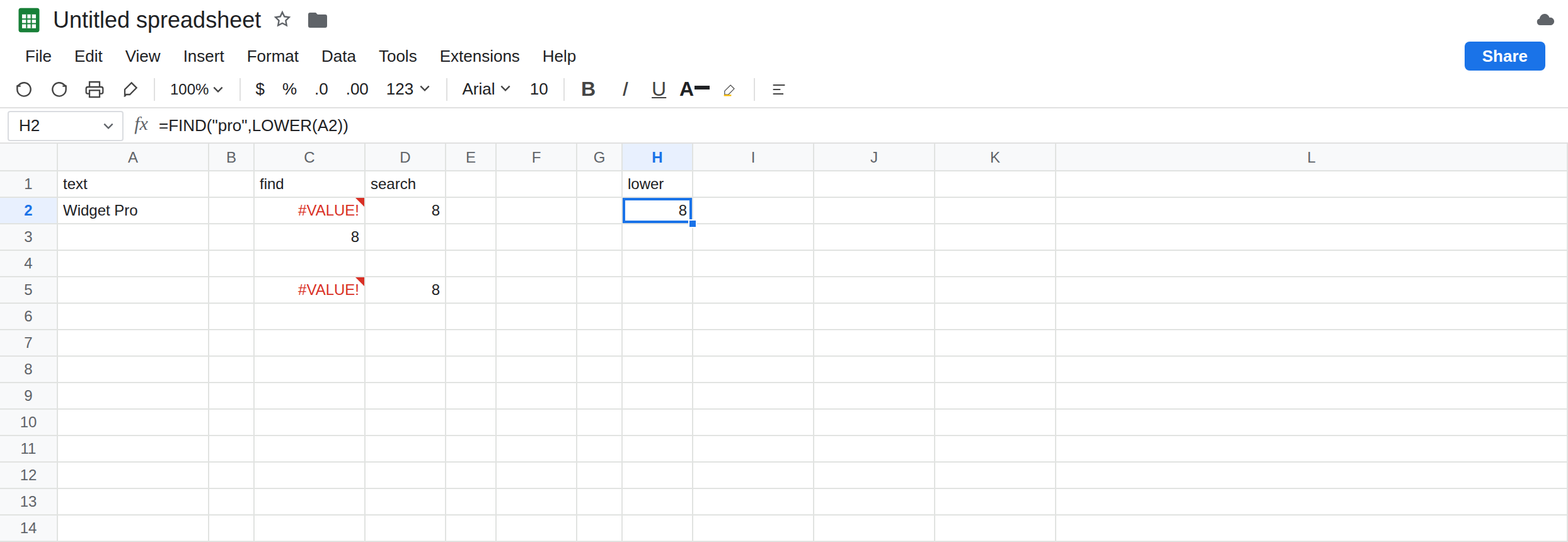
You care about case. Keep C3: =FIND("Pro",A2). Use the needle’s real capitals. In H2 enter =FIND("pro",LOWER(A2)). H2 is 8. LOWER is the fold. The needle pro is lowercase because LOWER made the haystack lowercase. Do not LOWER only one side.

You do not care about case, and the needle is plain text. Keep D2: =SEARCH("pro",A2). Do not pass a pattern with * unless you mean a wildcard.

The needle contains a star or a question mark. Use FIND when those marks are letters. Use SEARCH with a tilde (~*, ~?) when you must stay case-insensitive and still match the mark itself. A wildcard you did mean stays unescaped: D5.

Do not wrap C2 in IFERROR so a case miss becomes 0. Position 0 is not a real start, and the next MID will be wrong. See IFERROR vs IFNA. IFNA does not catch #VALUE!.

If FIND is #VALUE! and SEARCH of the same needle returns a number, the case differs or you passed ? or * to FIND. If both are #VALUE!, the substring is not there; use the miss page. If the number is past the end of the string you thought you had, check the third argument.

FIND vs SEARCH vs a folded FIND

FIND("pro") on Widget Pro is #VALUE!. SEARCH("pro") is 8. FIND("Pro") is 8. SEARCH("P?o") is 8 and FIND("P?o") is #VALUE!. FIND("pro", LOWER(text)) is the case-insensitive literal search. EXACT returns TRUE or FALSE, not a position. A start position after the only match is #VALUE! in whichever function you called.