SUMPRODUCT returns #VALUE! when the arrays are different sizes

SUMPRODUCT multiplies matching positions and adds those products. The arrays must be the same height and the same width. Three rows times four rows is #VALUE!. A column times a row, even with the same count of cells, is #VALUE!. The function returns one number when the shapes agree. It does not spill, and it does not recycle the shorter list.

This page is that size error. It is not MMULT dimensions (inner dimensions of a matrix product). It is not COUNTIFS range size (criteria ranges versus the sum range). It is not FILTER range size. Keep the Google Sheets UI in English.

Recreate it on a blank sheet

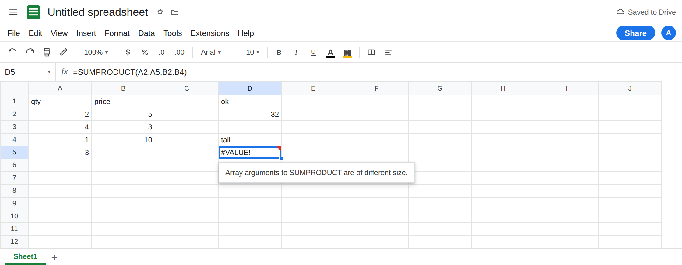
1. Open a blank spreadsheet. In A1 type qty, B1 price. A2 2, B2 5. A3 4, B3 3. A4 1, B4 10. A5 3. Leave B5 blank. Column A has four qtys. Column B has three prices.

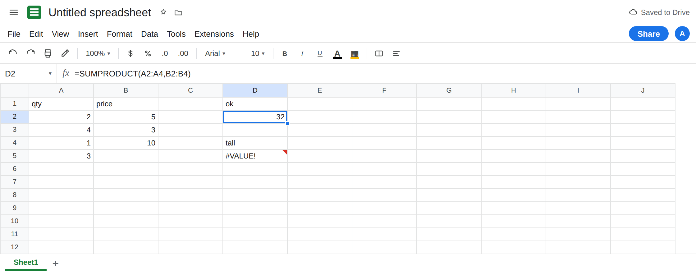
Matched rows. In D1 type ok. In D2 enter =SUMPRODUCT(A2:A4,B2:B4). D2 is 32 (2×5 + 4×3 + 1×10). That cell is the control. One number, no spill.

One extra row. In D4 type tall. In D5 enter =SUMPRODUCT(A2:A5,B2:B4). A2:A5 is four cells. B2:B4 is three. The cell shows #VALUE!. The tooltip is Array arguments to SUMPRODUCT are of different size. Leave D5 broken.

Column times row. In D7 enter =SUMPRODUCT(A2:A4,B2:D2). A2:A4 is 3×1. B2:D2 is 1×3. Both contain three cells. The orientations differ. D7 is #VALUE! with the same size tooltip. Leave D7 broken. SUMPRODUCT does not turn that pair into a dot product by rotating one side.

A condition range that is taller. In F1 type dock. F2 East. F3 West. F4 East. F5 East. In D9 enter =SUMPRODUCT((F2:F5="East")*(A2:A4)). The boolean array is four rows. The qty array is three. #VALUE! again. People write this to sum East qtys. The parentheses do not relax the shape. Leave D9 broken.

Text inside a matched shape is not this error. In C2 type 5, C3 3, C4 pcs. In H4 enter =SUMPRODUCT(A2:A4,C2:C4). The rectangles are both three rows by one column. H4 is 22 (2×5 + 4×3 + 1×0) with no error triangle. pcs counted as zero. That is a short total, not #VALUE!. Leave H4 as 22 so you can see the quiet zero. A vertical array literal uses semicolons on a US locale ({5;3;0}). If { } is Formula parse error, the separator rules are array literal locale. Do not debug H4 as a size error.

Leave D5, D7, and D9 broken. Leave D2 as 32.

What is actually wrong

• Every array in one SUMPRODUCT must share one rectangle. Height and width are both checked. “Same number of cells” is not enough when one range is a row and the other is a column. D7.
• Open-ended ranges drift. A2:A and B2:B are the same height (the rest of the sheet). A2:A and B2:B100 are not, once the sheet is taller than row 100. D5 is the short version of that mistake: A runs through row 5, B stops at row 4.
• Boolean conditions have to be built on the same rows as the values. (F2:F5="East") is four booleans. Multiplying by A2:A4 never pairs East on row 5 with a qty. The error is the size tooltip, not a wrong dock total.
• Text and blanks in a matching rectangle become 0 in the product. H4 is 22, not #VALUE!. If you expected #VALUE! from pcs, you are thinking of SUM of a text cell in some other formulas, or of wrong type (10+pcs). SUMPRODUCT coerces text to zero and keeps going. A short total with no triangle is that coercion. A triangle with the size sentence is D5.
• SUMPRODUCT returns one cell. A #REF! means something else (a deleted reference inside the formula), not a spill. See after you delete.

This is not MMULT. MMULT wants the inner dimensions to agree so it can spill a matrix. See MMULT dimensions. Feeding MMULT these two columns is a different #VALUE!.

Fix

Leave D5, D7, and D9 broken.

Use the same rows. Keep D2: =SUMPRODUCT(A2:A4,B2:B4) is 32. If A5 should count, put a price in B5 first, then =SUMPRODUCT(A2:A5,B2:B5). Do not stop one range a row early.

Same orientation. To weight a column, pass two columns. To weight a row, pass two rows: =SUMPRODUCT(A2:C2,A3:C3) after you put a price row in row 3. Do not pass A2:A4 with B2:D2 and expect Sheets to transpose one of them. Wrap one side in TRANSPOSE only when you mean that rotation: =SUMPRODUCT(A2:A4,TRANSPOSE(B2:D2)) if B2:D2 really holds the three prices.

East qty, same height. =SUMPRODUCT((F2:F4="East")*(A2:A4)) pairs three docks with three qtys. F5 is outside that call. Or use SUMIF, which is built for one criteria column. See SUMIFS date text for a different SUMIFS miss. Do not wrap D5 in IFERROR. See IFERROR vs IFNA.

If the tooltip says the array arguments are of different size, count rows and columns on each argument, not the number of filled prices. If the total is quietly short and pcs sits in a matched cell, that cell became zero. That is not the size error.