

ISNA of a column returns one FALSE unless you array-enter it
Updated
ISNA answers one question: is this value #N/A? Pass it A2:A without ARRAYFORMULA and Sheets answers for the first cell only. One FALSE. The #N/A in A4 never gets a turn. A filter or an IF built on that single FALSE treats the whole column as clean.
What the three flags mean on one cell is ISERROR vs ISNA. AND / OR collapsing a range to one boolean is ARRAYFORMULA AND/OR. This page is ISNA on a range. Keep the Google Sheets UI in English.
Recreate it on a blank sheet
Section titled “Recreate it on a blank sheet”- Open a blank spreadsheet. In A1 type
sku. A2101. A3102. In A4 enter=NA(). A4 is#N/A. A5104. The miss is not in the first row.
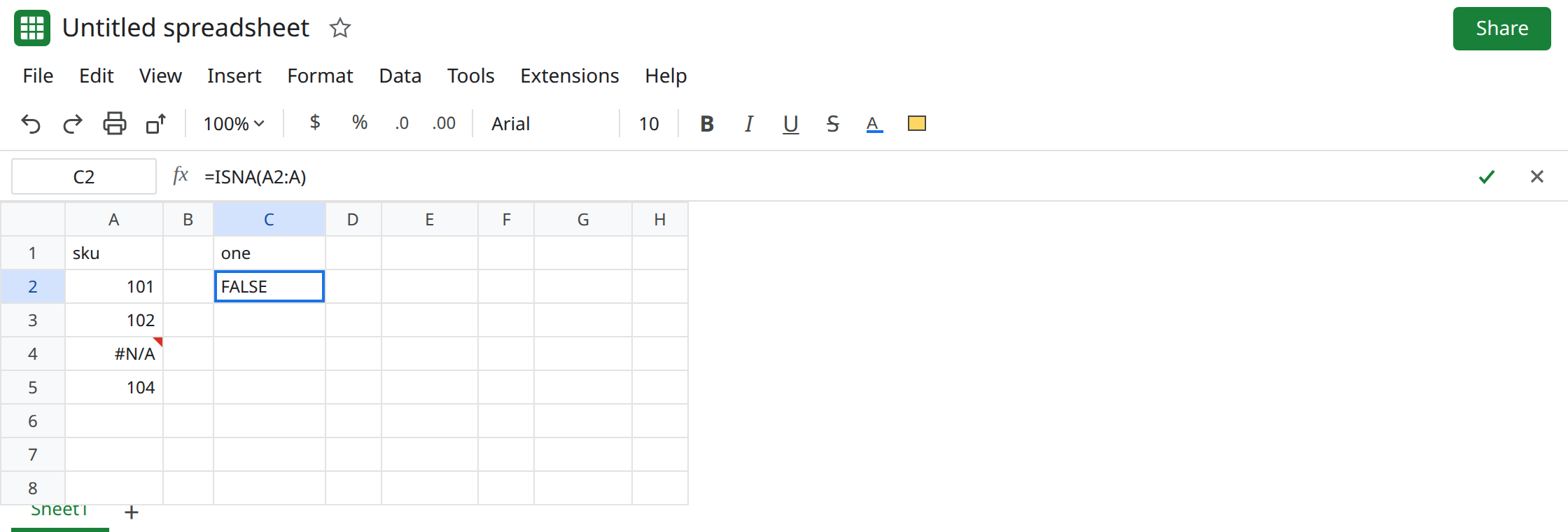
One ISNA on the range. In C1 type one. In C2 enter =ISNA(A2:A). C2 is FALSE. One cell. A4 is #N/A and C2 does not mention it. =ISNA(A2:A5) is the same FALSE, because A2 is 101, and ISNA of a number is FALSE. Leave C2 as that single FALSE.
The first cell can flip the one flag and still hide the rest. In A8 enter =NA(). In C8 enter =ISNA(A8:A10). C8 is TRUE. One cell. Put 101 in A9. C8 stays TRUE. You have not learned whether A9 is a miss. You have learned that A8 is #N/A. Leave C8 as that single TRUE.
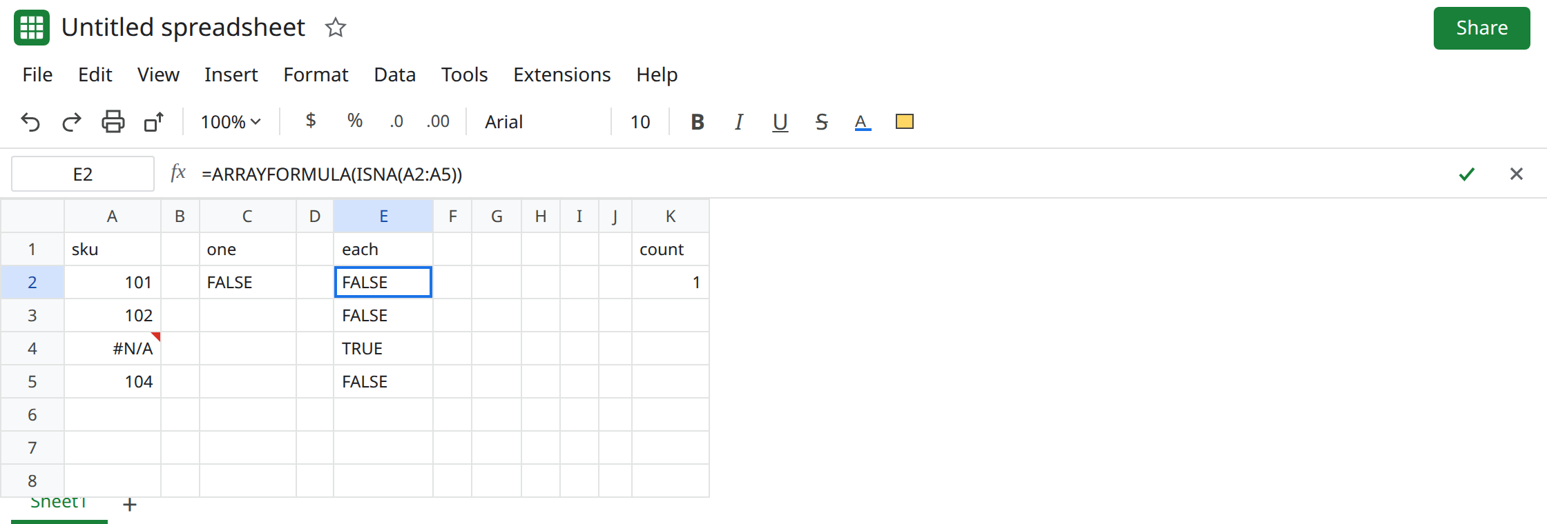
Per-row flags. In E1 type each. In E2 enter =ARRAYFORMULA(ISNA(A2:A5)). E2 is FALSE, E3 is FALSE, E4 is TRUE, E5 is FALSE. Four answers. A4’s #N/A is visible. Leave E2 as the control.
ISERROR on the same range, same shape. In G2 enter =ISERROR(A2:A5). G2 is FALSE. One cell, the first row, even though A4 is an error. =ARRAYFORMULA(ISERROR(A2:A5)) spills FALSE, FALSE, TRUE, FALSE. The array habit is not special to ISNA. The meaning of each flag is ISERROR vs ISNA. ISERROR is TRUE for #DIV/0! as well. ISNA is not.
A count from the single FALSE. In I1 type count. In I2 enter =COUNTIF(C2,TRUE). I2 is 0. You counted the one flag, not the column. That zero is not “no #N/A in A.” Leave I2 as 0.
What is actually wrong
Section titled “What is actually wrong”- Without
ARRAYFORMULA(or another array caller such asSUMPRODUCT/MAP),ISNAdoes not spill. The value you see is the test of the top-left cell of the range. A2 is101. FALSE is correct for A2 and useless for A4. - An open range
A2:Adoes not mean “any row.” It still starts at A2. A blank A2 is also not#N/A, soISNAis FALSE while a miss sits below the blank. IF(ISNA(A2:A),"missing",A2:A)withoutARRAYFORMULAtakes one branch for the first cell. It does not label A4. WithARRAYFORMULAit can spill, and the false branch still returns#N/Aon the miss row if you pass the original cell through. Test and branch per row on purpose.AND(ISNA(A2:A5))is one boolean for another reason. See ARRAYFORMULA AND/OR. C2 isISNAitself returning one FALSE, notAND.
This is not IFNA, which replaces #N/A with another value. See IFERROR vs IFNA. C2 does not change A4. A4 stays #N/A.
Leave C2 as the single FALSE and A4 as #N/A.
Spill the test. Keep E2: =ARRAYFORMULA(ISNA(A2:A5)). In K2 enter =COUNTIF(E2:E5,TRUE). K2 is 1. That count sees A4. =SUMPRODUCT(ISNA(A2:A5)*1) is also 1, because SUMPRODUCT evaluates the range as an array even without ARRAYFORMULA. Use one of those, not COUNTIF on C2.
Per row with MAP. =MAP(A2:A5,LAMBDA(v,ISNA(v))) spills the same four flags. Use it when the test sits next to other lambda logic.
Do not wrap A4 in IFNA and then ISNA the wrapper. The flag would be FALSE because the #N/A is already gone. See IFERROR hides cause.
If ISNA of a range is one FALSE, it tested the first cell. Array-enter it before you treat that FALSE as a clean column. If the first cell is #N/A and the flag is a single TRUE, the rows under it are still untested.