FREQUENCY spills one row past the bins, and a filled cell is #REF!

FREQUENCY(data, classes) counts how many values fall into each bin. The bins are the class limits you list, in ascending order. The result is a vertical array with one more row than you have bins. The last row counts values greater than the last limit. Two bins produce three numbers. If any of those rows is already filled, the formula shows #REF! and the tooltip says the array result was not expanded because it would overwrite data. Bins that are out of order do not always error. They count into the wrong slots, and the total can still add up.

A blocked spill is the same mechanic as MODE.MULT spill and SORT / UNIQUE spill. Keep the Google Sheets UI in English. Sheet Error is an independent formula-error library, not a Google product.

Recreate it on a blank sheet

1. Open a blank spreadsheet. In A1 type v. A2 1. A3 3. A4 5. A5 7. A6 12. Five values. In B1 type bin. B2 4. B3 8. Two limits, ascending.

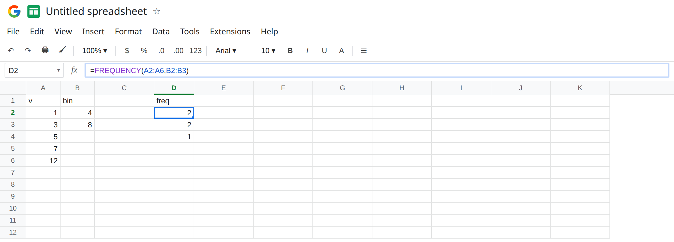
A clear spill. In D1 type freq. In D2 enter =FREQUENCY(A2:A6,B2:B3). D2 is 2 (values ≤ 4: the 1 and the 3). D3 is 2 (values > 4 and ≤ 8: the 5 and the 7). D4 is 1 (values > 8: the 12). Three cells. 2+2+1 is 5, every input accounted for. D5 is empty. That block is the control.

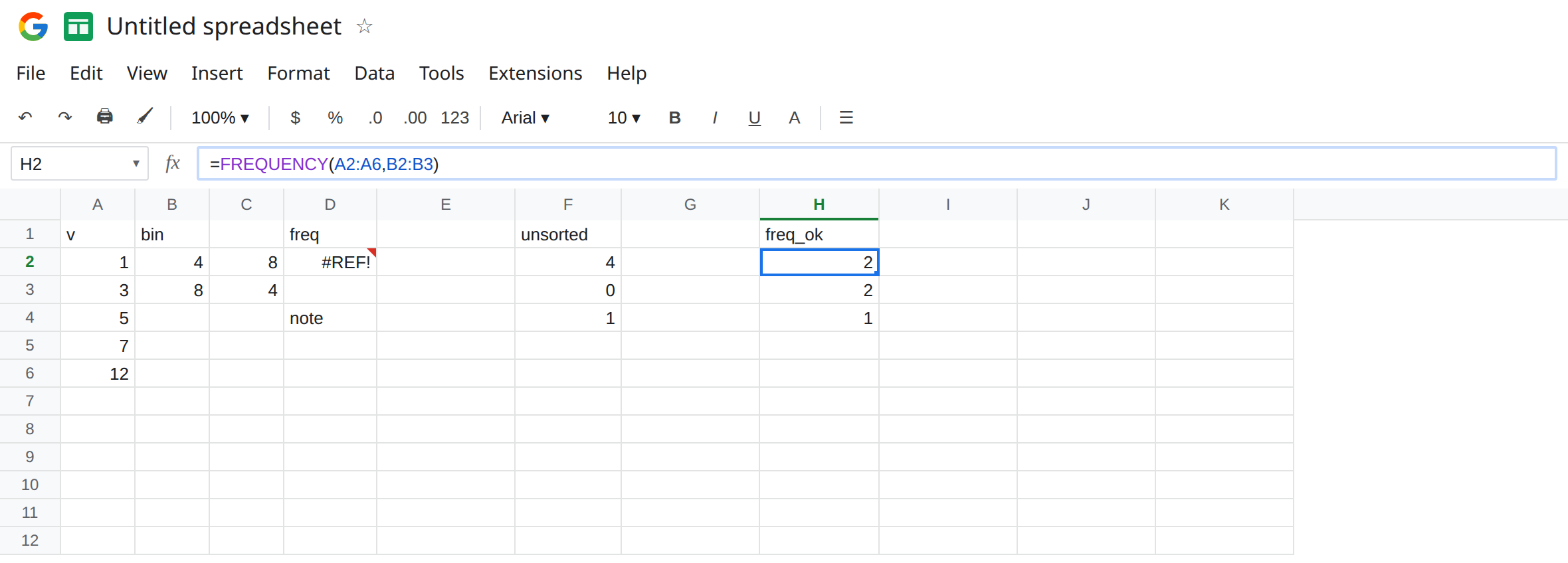
Block the extra row. In D4 type note. D4 was the “greater than 8” count. D2 becomes #REF!. The tooltip names D4 as the cell that would be overwritten. The bins did not become illegal. The third count has nowhere to go. People who budget “two rows because I have two bins” always collide with this extra row. Leave note in D4 and leave D2 as #REF!.

Unsorted bins, no triangle. Move to column F so the broken spill stays. In F1 type unsorted. In C2 type 8 and C3 type 4 — high limit first. In F2 enter =FREQUENCY(A2:A6,C2:C3). The first bin is “≤ 8,” which already catches 1, 3, 5, and 7. That count is 4. The second bin is “> 8 and ≤ 4,” which is empty, so 0. The last row is 1 (the 12, which is greater than the last limit in the list). F2:F4 is 4, 0, 1. No #REF! and no #NUM!. The total is still 5. The histogram is wrong if you label F2 as “≤ 4.” FREQUENCY walks the class list in the order you wrote, and it does not sort it for you.

Leave D2 as #REF!. Leave F2:F4 as 4, 0, 1. The numeric classes are B2:B3. Including the header bin in the class range changes how many numeric limits FREQUENCY sees.

What is actually wrong

• Output rows = number of numeric class limits + 1. The extra row is “greater than the last class,” not an error and not an optional total. If you need a total, sum the spill. Do not add a bin to create it.
• The overwrite is #REF! on the formula cell, same as any spill. Clearing a cell below the spill does nothing if the occupied cell is inside it. Here the inside cell is the third row.
• Unsorted classes still return counts. The first class catches everything up to its limit, even when a later class is a smaller number. You get zeros in the later bins and a quiet wrong chart.
• Duplicate class limits produce a bin that nothing new can fall into (the “greater than previous and ≤ this” slice has zero width). The count is 0 for that slice. It is not #NUM!.
• Blank data cells are ignored. They are not a bin. Text in the data is ignored. A column of mixed labels changes the counts without a triangle. 12 stored as text will not land in the last bin.

This is not COUNTIFS with "<="&4. You can rebuild this histogram with COUNTIFS, and those ranges have their own size rule. See COUNTIFS range size. FREQUENCY’s bug on this page is the spill height and the bin order.

This is not PERCENTILE #NUM!. See PERCENTILE.EXC bounds.

Fix

Leave D4 as note so the #REF! stays. Leave the unsorted example in F2.

Reserve one extra row and sort the limits ascending. In H1 type freq_ok. In H2 enter =FREQUENCY(A2:A6,B2:B3). H2 is 2, H3 is 2, H4 is 1. Nothing is typed in H2:H4 except the formula in H2. Put notes in H6 or in another column.

Sort the class list. B2 4, B3 8, not 8 then 4. If the limits come from a column people edit, wrap them in SORT only when you are sure a sorted copy is what FREQUENCY should see: =FREQUENCY(A2:A6,SORT(B2:B3)). A sort fixes order. It does not fix a blocked spill.

Label the last row > last bin so nobody deletes it as a stray #N/A. It is a count. On this sheet it is 1.

Do not wrap D2 in IFERROR. You would hide the collision and show a blank histogram. Move note. See IFERROR vs IFNA.

If FREQUENCY is #REF!, you have one fewer empty row than bins+1. If the counts sum to the number of numeric inputs but the first bin looks too big, the class list is not ascending. If a value you can see is missing from every bin, it is text, not a number.

Three rows, two bins

Bins 4 and 8, data 1, 3, 5, 7, 12: the spill is 2, 2, 1. The third number is the 12. A note in that third cell makes the formula #REF!. Bins 8 then 4 spill 4, 0, 1 with no error. The extra row is part of the result, not an overflow.