

Fix INDEX #REF! in Google Sheets (row or column past the range)
Updated
INDEX returns a cell (or a whole row / column) from a range by position. #REF! here means the position you asked for is not inside that range. The formula bar still shows INDEX and a real range. Nothing was deleted. The index is too big.
This page is INDEX past the range. It is not VLOOKUP bad index (the third argument of VLOOKUP counted from the left of the lookup block). It is not after you delete (#REF! inside the formula text). It is not INDIRECT #REF! (text that is not a valid address).
Recreate it on a blank sheet
Section titled “Recreate it on a blank sheet”- Open a blank spreadsheet. In A1 type
sku, B1name. A2101, B2Widget. A3102, B3Gadget. A4103, B4Lamp. That data range is three rows by two columns:A2:B4. - Row index too big. In D1 type
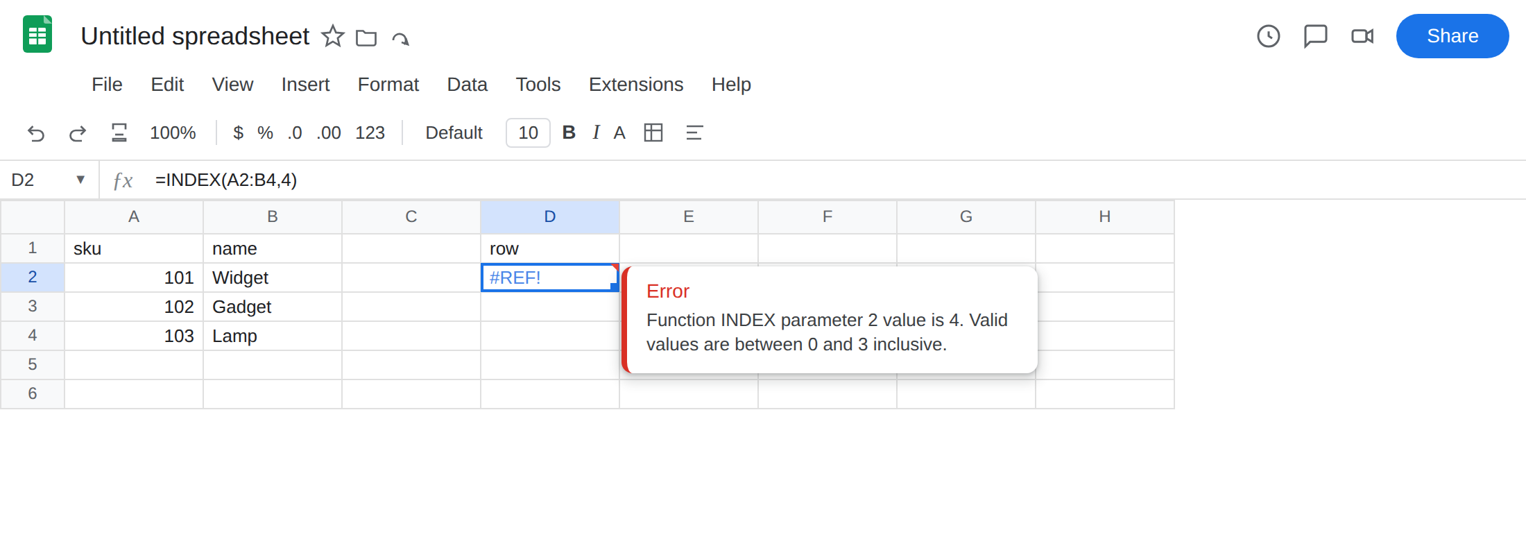
row. In D2 enter=INDEX(A2:B4,4). The cell shows#REF!.A2:B4has rows 1, 2, and 3 relative to the range (A2, A3, A4). Index4asks for a fourth row that range does not have. Leave D2 broken.
- Column index too big. In D4 type
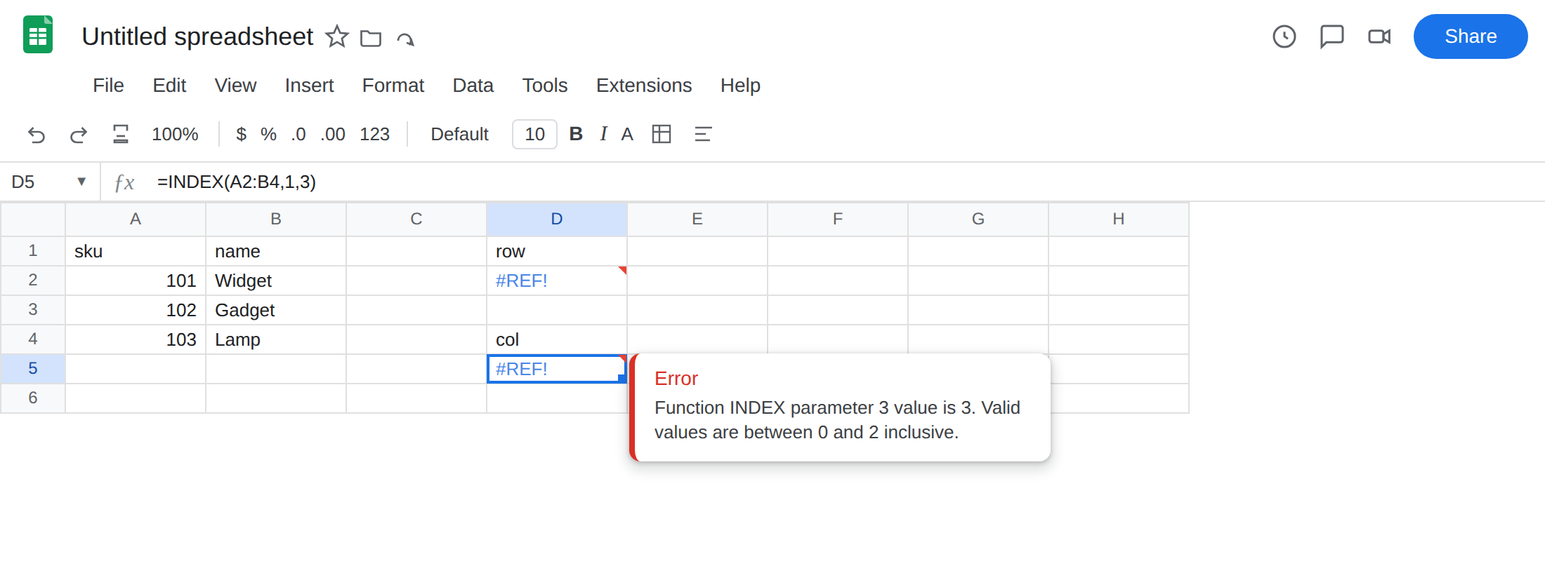
col. In D5 enter=INDEX(A2:B4,1,3). The cell shows#REF!. The range is two columns wide (sku, name). Index3asks for a third column. Row1would have been legal on its own (INDEX(A2:B4,1)is101). The optional column argument is what breaks it. Leave D5 broken.
- A control that fits. In D7 type
ok. In D8 enter=INDEX(A2:B4,2,2). The cell shows Gadget. Relative row 2 is A3/B3. Relative column 2 is name. Same function, legal indexes.
Select D2 and read the formula bar. It is still =INDEX(A2:B4,4). There is no #REF! token inside the formula. That is the tell versus a delete.
Zero and blank. In F1 type zero. In F2 enter =INDEX(A2:B4,0). In Sheets, row 0 (and a blank row argument in some forms) can mean “the whole column / all rows,” not an error. Do not treat F2 as this #REF!. This page is an index past the last row or column, not 0. If F2 spills or returns a column, that is expected. Leave D2 as the broken one.
What is actually wrong
Section titled “What is actually wrong”INDEX(range, row, [column])counts from the top-left of that range, starting at 1.INDEX(A2:B4,4)is not “spreadsheet row 4.” Spreadsheet row 4 is Lamp, which is relative row 3. Relative row 4 does not exist.#REF!.INDEX(A2:B4,1,3)is relative column 3. The range stops at B. Column C is on the sheet. It is outside the range you passed. Same error value as the oversized row.- The tooltip is an out-of-range index, not Circular dependency detected, not Array result was not expanded, not You need to connect these sheets.
INDEXof a single column (INDEX(A2:A4,2)) has no column argument to overflow.INDEX(A2:A4,2,2)is#REF!because that range is one column wide.
This is not VLOOKUP column index #REF!. =VLOOKUP(101,A2:B4,3,FALSE) is also #REF!, but the third argument is a VLOOKUP index into the lookup block, and the formula is VLOOKUP. See VLOOKUP bad index. HLOOKUP does the same with a row index. See HLOOKUP #N/A / #REF!. Do not copy a VLOOKUP index fix onto INDEX without counting relative row and column separately.
This is not a deleted cell. After a delete, the formula bar contains #REF! (=A1+#REF!). See after you delete. D2 still names A2:B4.
This is not INDIRECT. =INDIRECT("not an address") is #REF! because the string is not A1. See INDIRECT #REF!.
This is not a SORT / UNIQUE spill, not OFFSET walking off the grid, and not a circular loop. See SORT / UNIQUE spill, OFFSET #REF!, circular dependency.
This is not #N/A. If the indexes are legal and you wrapped MATCH around a missing key, you would get #N/A from MATCH, not #REF! from INDEX. See MATCH #N/A.
Leave D2 and D5 broken so #REF! stays on the sheet.
Use a row that exists. In G1 type row_ok. In G2 enter =INDEX(A2:B4,3). The cell shows 103 (first column of relative row 3). For Lamp: =INDEX(A2:B4,3,2). If the row index comes from MATCH, keep MATCH exact (0) and wrap IFNA on MATCH, not IFERROR on INDEX. A bad INDEX row should stay #REF! until you fix the number.
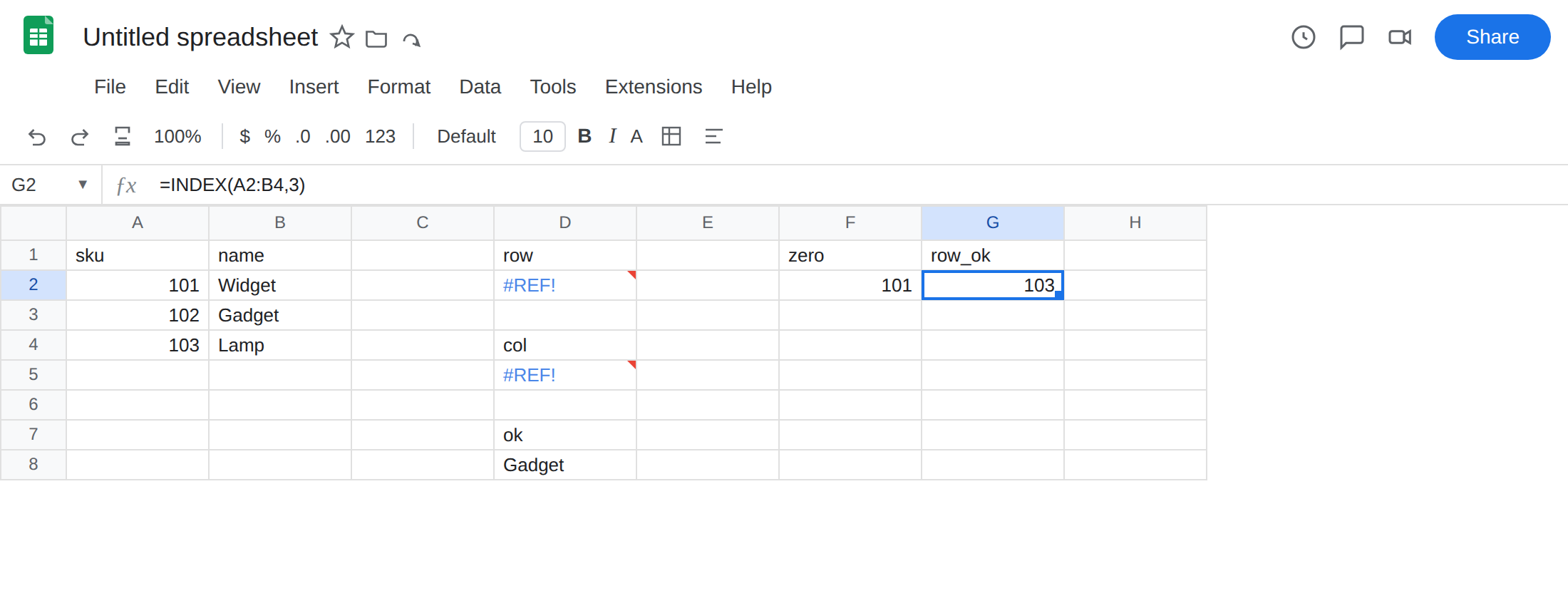
Use a column that exists. In G5 enter =INDEX(A2:B4,1,2). The cell shows Widget. Column 2 is name. There is no column 3 in A2:B4. Widen the range only if you truly need a third field: =INDEX(A2:C4,1,3) after you put a price in C.
Count from the range, not from A1. INDEX(B2:B4,1) is Widget, not 101. Relative row 1 of B2:B4 is B2.
Do not wrap this #REF! in IFNA. IFNA will not catch it. IFERROR will print none for a bad index as if a lookup missed. See IFERROR vs IFNA. Fix the indexes.
If INDEX is #REF! and the formula still reads INDEX with a real range, the row or column number is past that range. Shrink the index, or widen the range to match the index you meant.