

Fix EOMONTH #NUM! in Google Sheets (start date unparseable or months overflow)
Updated
EOMONTH returns the last day of the month that is months away from a start date. #NUM! means the start is not a date serial this file can use, or the result would sit outside the dates Sheets can represent. The formula parsed. The calendar math cannot land.
This page is EOMONTH #NUM!. It is not DATEVALUE locale (DATEVALUE of 13/1/2024 on a US locale is #VALUE!). It is not out of domain (SQRT(-1)). It is not WORKDAY #NUM! or NETWORKDAYS #NUM!. Keep the Google Sheets UI in English.
Recreate it on a blank sheet
Section titled “Recreate it on a blank sheet”- Open a blank spreadsheet. File → Settings. Display language English. Locale United States so the DATEVALUE contrast below matches. In A1 type
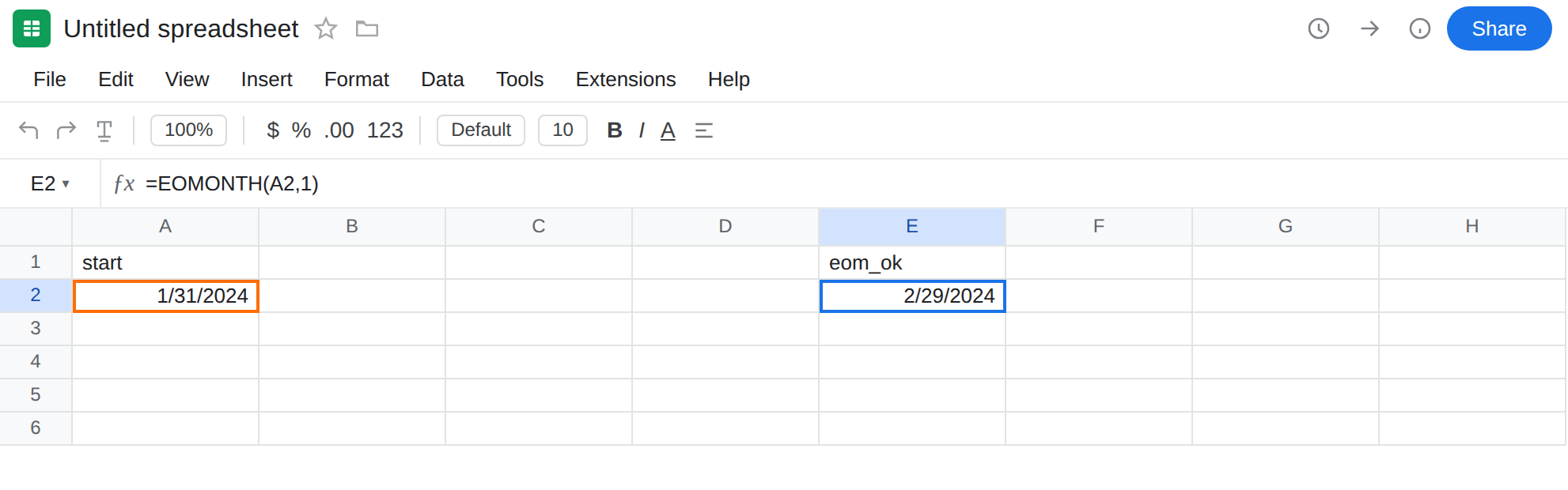
start. In A2 enter=DATE(2024,1,31).
A month-end the function can return. In E1 type eom_ok. In E2 enter =EOMONTH(A2,1). The cell is the last day of February 2024 (2/29/2024 — 2024 is a leap year). Format E2 as a date if you only see a serial. That row is the control: real start, modest months.
Impossible start serial. In E4 type bad_serial. In E5 enter =EOMONTH(4000000,0). The cell shows #NUM!. 4000000 is a number. It is not a date this calendar will treat as start_date. Leave E5 broken.
Months overflow. In E7 type overflow. In E8 enter =EOMONTH(A2,200000). The cell shows #NUM!. January 2024 plus two hundred thousand months is past the last date Sheets will return. Leave E8 broken.
DATEVALUE contrast — different error. In G1 type dmy. In G2 type an apostrophe then 13/1/2024. In G3 enter =DATEVALUE(G2). The cell shows #VALUE! on United States (month 13). That is unparsable text for DATEVALUE. It is not EOMONTH. Leave G3 as the contrast. See DATEVALUE locale.
Text start on EOMONTH. In G5 enter =EOMONTH("soon",0). This is #VALUE! (wrong type / unparsable text), not #NUM!. This page’s “unparseable start” is an impossible serial — a number that is not a date — plus months that overflow. Stay on E5 and E8 for #NUM!.
Leave E5 and E8 as the broken formulas. Leave E2 as 29 Feb 2024.
What is actually wrong
Section titled “What is actually wrong”EOMONTH(start_date, months)needs a start that is a real date serial (or a value Sheets can coerce to one) and a result still inside the spreadsheet calendar.4000000fails the first test.200000months fails the second. Both are#NUM!.monthsmay be negative (go backward). A huge negative month count overflows the other end of the calendar the same way.#NUM!.EOMONTHof a legal date always returns a month-end, not “same day-of-month next month.”DATE(2024,1,31)plus one month is 29 Feb 2024, not 31 Feb. That control is E2. It is not an error.- The tooltip names
EOMONTHand a numeric domain problem. It is not Unable to parse query string, not Unknown function, not DATEVALUE parameter … cannot be parsed to date/time (that sentence is G3).
This is not DATEVALUE of locale-shaped text. 13/1/2024 on a US file is #VALUE!. See DATEVALUE locale. Do not change File → Settings → Locale to repair E5. E5 never parsed a string.
This is not SQRT of a negative. See out of domain. Same error value, different function.
This is not WORKDAY / NETWORKDAYS weekend 99. See WORKDAY #NUM! and NETWORKDAYS #NUM!. EOMONTH has no weekend code.
This is not #VALUE! from "soon" or 10 + pcs. See wrong type. G5 is that family. E5 is a number the date system rejected.
Leave E5 and E8 broken so #NUM! stays on the sheet. Leave E2 as the working month-end.
Pass a real start date. Prefer DATE(year, month, day) or a cell that already holds a date. In F5 enter =EOMONTH(A2,0). The cell is 1/31/2024 (last day of the start month). Do not point start_date at a leftover id, a row number, or 4000000.
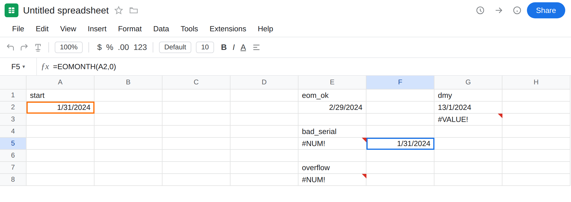
Shrink months. In F8 enter =EOMONTH(A2,1). The cell matches E2. If months comes from a cell, sanity-check it (=IF(ABS(B2)>1200,"",EOMONTH(A2,B2)) or whatever window your invoices actually use). You cannot EOMONTH your way to year 200000.
Convert text dates before EOMONTH. If the start is leftover text that this locale can parse, =EOMONTH(DATEVALUE(G2),0) still fails on G2 because G2 is 13/1/2024 on US. Fix the string or use =EOMONTH(DATE(2024,1,13),0). Do not wrap E5 in DATEVALUE — DATEVALUE(4000000) is not a locale-text problem.
Do not wrap E5 in IFERROR and call the close date fixed. You still do not have a month-end. See IFERROR vs IFNA. IFNA will not catch #NUM!.
If EOMONTH is #NUM!, check ISNUMBER on the start, then whether the start is a plausible date (TO_DATE / format as date), then whether months is a realistic offset. Locale text that fails to parse is #VALUE! on DATEVALUE — different primer.
EOMONTH vs DATEVALUE vs EDATE
Section titled “EOMONTH vs DATEVALUE vs EDATE”DATEVALUE turns text into a date with this spreadsheet’s locale. Failure is #VALUE!. See DATEVALUE locale. EOMONTH does not pick M/D/Y vs D/M/Y for you. Feed it a date, not a string you have not parsed.
EDATE(start, months) returns the same day-of-month offset (clamped), not necessarily month-end. EDATE of an impossible serial is the same #NUM! family. If you wanted last-of-month invoices, keep EOMONTH. If you wanted “31 Jan plus one month as a same-day-ish date,” EDATE is the other function — and 31 Jan plus one month still will not invent 31 Feb.
DATE(year, month+1, 0) is an old pattern for last-of-month. DATE rolls overflowing months instead of #NUM! (DATE(2024,13,1) is 1 Jan 2025). Prefer DATE for parts you already split, EOMONTH when the input is already a date and months stays on the calendar.