FILTER returns #N/A when any criteria cell is #N/A

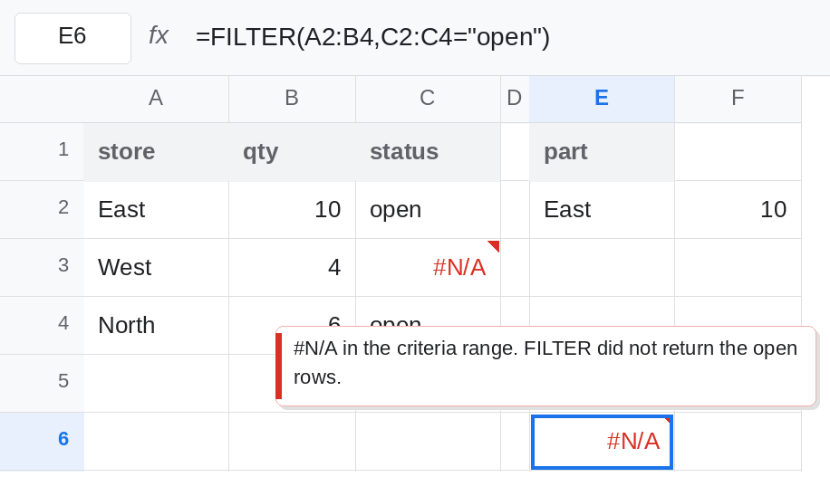
FILTER(range, condition) keeps rows where condition is TRUE. The condition has to be a boolean for every row. If any cell in that condition is #N/A, the condition is not a clean list of TRUE and FALSE. FILTER returns #N/A for the whole spill. Rows that really were open do not appear. The tooltip is about the #N/A in the criteria, not about “no matches.” Replacing the error inside the condition with FALSE lets the other rows through. Wrapping the entire FILTER in IFNA hides this bug and also hides a real empty result.

No matching rows, when every condition cell really is FALSE, is FILTER no match. A condition range of the wrong height is FILTER range size. IFNA versus IFERROR on spills is IFNA vs IFERROR spill. Keep the Google Sheets UI in English. Sheet Error is an independent formula-error library, not a Google product.

Recreate it on a blank sheet

1. Open a blank spreadsheet. In A1 type store, B1 qty, C1 status. A2 East, B2 10, C2 open. A3 West, B3 4. In C3 enter =NA(). C3 is #N/A. A4 North, B4 6, C4 open. Two rows are open. One status cell is an error. The quantities you want are East 10 and North 6.

A condition with no error. In E1 type part. Leave E2:F3 empty. In E2 enter =FILTER(A2:B2,C2:C2="open"). One row, and that row is open. The spill is East and 10. In E4 enter =FILTER(A4:B4,C4:C4="open"). North and 6. Each call avoided C3. Those two spills are the control.

The full column, one bad cell. In E6 enter =FILTER(A2:B4,C2:C4="open"). The cell shows #N/A. East and North never spill. C2 and C4 are the text open. They do not get a vote once C3’s #N/A is inside the same condition. Leave E6 broken.

A lookup column does the same thing. In D2 enter =VLOOKUP(A2,{"East","open";"North","open"},2,FALSE). D2 is open. Fill D3. West is not in that little array, so D3 is #N/A. D4 is open. In E8 enter =FILTER(A2:B4,D2:D4="open"). E8 is #N/A again. You do not need =NA() typed by hand. A VLOOKUP miss in the criteria column is enough. Leave E8 broken. That miss on its own is VLOOKUP no match.

Every status FALSE is a different #N/A. In E10 enter =FILTER(A2:B4,C2:C4="shut"). Nothing is shut, and C3 is still #N/A, so this cell is #N/A for the error reason, not because you can see zero shut rows. You cannot read E10 until the #N/A in C3 is turned into a boolean. Do that in the fix, and then a real shut filter becomes the no-match #N/A from FILTER no match.

Leave E6 and E8 as #N/A. Leave E2 as East and 10.

What is actually wrong

• FILTER will not skip a bad criteria cell and continue. One #N/A fails the call. E6. The rows whose own status is open are included only when every element of the condition is TRUE or FALSE.
• The error is often one column over, in a lookup you meant as a helper. D3. Filtering A2:B4 does not insulate you from D2:D4.
• =NA() and a failed VLOOKUP are the same token inside the condition. Fixing the lookup, or catching it in the condition, both work. Leaving it and wrapping FILTER in IFNA does not tell you which row was bad.
• A condition that is entirely FALSE, with no errors, is also #N/A. That is “no rows,” and it is what E10 should become after C3 cannot leak. The two #N/A results look identical. The formula bar does not.
• #DIV/0! or #VALUE! in the criteria column fails the filter too. IFNA catches only #N/A. IFERROR catches the rest. Use the one that matches the token in the helper. See IFNA vs IFERROR spill.

This is not FILTER range size. A2:B4 and C2:C4 are the same height. The tooltip on E6 is not “expected row count.”

Fix

Leave E6 broken so the leaked #N/A stays visible.

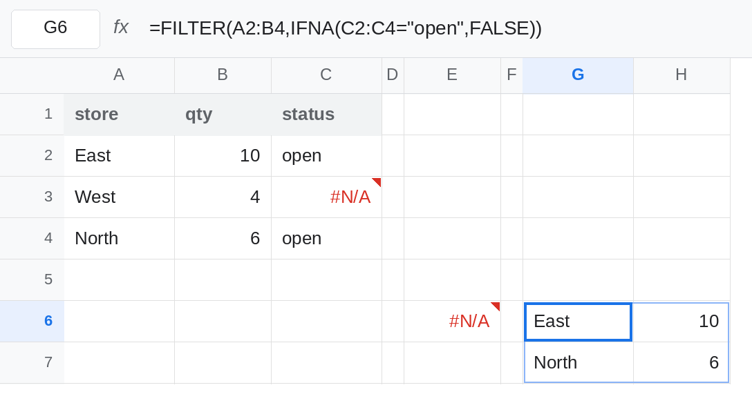
Turn each criteria error into FALSE. In G6 enter =FILTER(A2:B4,IFNA(C2:C4="open",FALSE)). G6 spills East / 10 and North / 6. West drops out, because #N/A became FALSE, which is what “this row did not pass” means. You do not need ARRAYFORMULA around IFNA here. FILTER evaluates the condition as an array. For the lookup helper, =FILTER(A2:B4,IFNA(D2:D4="open",FALSE)) is the same shape.

Or fix the helper so it cannot be #N/A. In D2 use =IFNA(VLOOKUP(A2,{"East","open";"North","open"},2,FALSE),"") and fill down. D3 is blank instead of #N/A. Then =FILTER(A2:B4,D2:D4="open") spills East and North without IFNA inside FILTER. Blank is not open. The row drops. That is XLOOKUP blank fallback if the helper should be XLOOKUP instead of VLOOKUP.

After the condition is clean, trust a remaining #N/A. =FILTER(A2:B4,IFNA(C2:C4="shut",FALSE)) is #N/A because no row is shut. That one you may replace with a message using IFNA around the whole FILTER. Do not put that wrapper on E6 first. You would hide C3.

If FILTER is #N/A and a criteria cell shows an error triangle, the match is not empty yet. Catch the error inside the condition, or remove it from the helper. If every criteria cell is FALSE and none are errors, the #N/A is FILTER no match.