LOOKUP in vector form returns the next smaller key and does not say the key was missing

LOOKUP(search_key, search_range, result_range) is the vector form. It expects search_range sorted ascending. If the key is there, you get that row. If the key is not there, you get the largest key that is still smaller, and no error. On 10, 20, 30, 40, a lookup of 25 returns the name beside 20. VLOOKUP of 25 with FALSE is #N/A. LOOKUP has no FALSE argument. The array form, one range and no separate result vector, searches the first column or the first row by shape and returns the last column or the last row. That is a different call.

Approximate VLOOKUP is VLOOKUP wrong row and VLOOKUP TRUE bands. Approximate MATCH is MATCH approx unsorted. Exact XLOOKUP is XLOOKUP #N/A. Keep the Google Sheets UI in English. Sheet Error is an independent formula-error library, not a Google product.

Recreate it on a blank sheet

1. Open a blank spreadsheet. In A1 type qty, B1 name. A2 10, B2 Desk. A3 20, B3 Chair. A4 30, B4 Lamp. A5 40, B5 Sofa. The qty column is sorted ascending. These are quantity breaks, not skus.

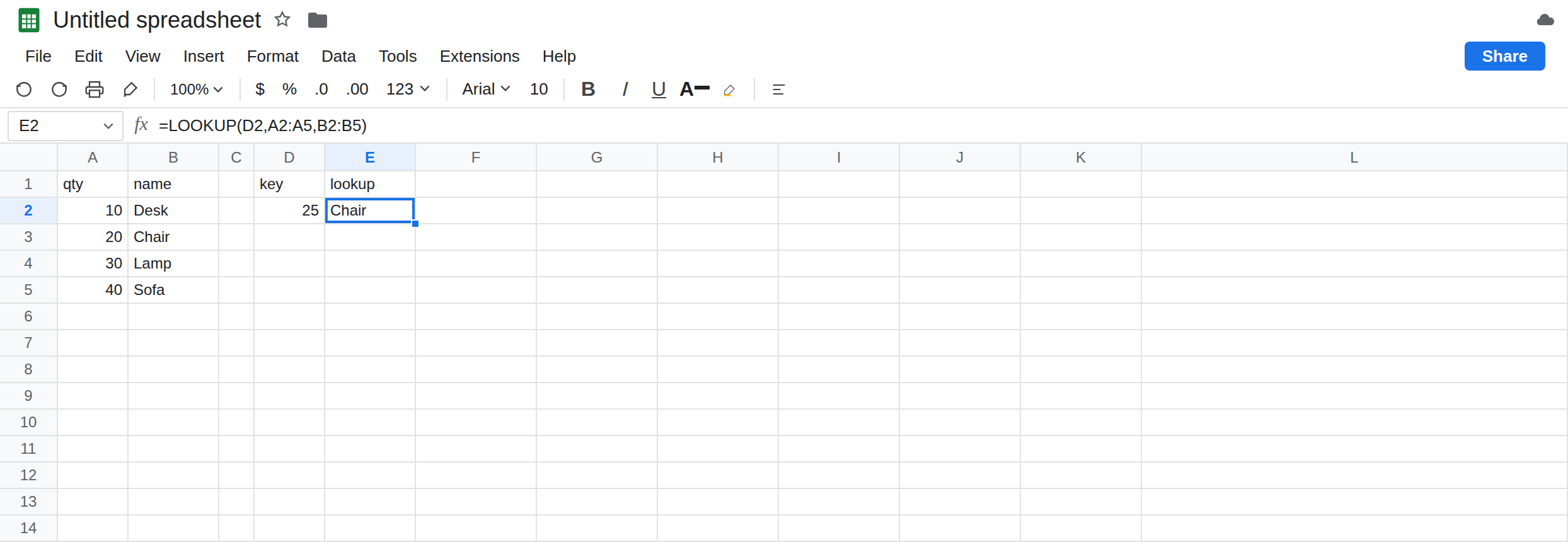
25 is not in the list. In D1 type key. D2 25. In E1 type lookup. In E2 enter =LOOKUP(D2,A2:A5,B2:B5). E2 is Chair. The largest qty that is still less than or equal to 25 is 20, and 20 is Chair. There is no triangle. Nothing in the cell says “approximate.” Leave E2 as Chair.

The neighbors that are exact or past the ends. In E4 enter =LOOKUP(20,A2:A5,B2:B5). E4 is Chair. An exact key returns that row. In E5 enter =LOOKUP(40,A2:A5,B2:B5). E5 is Sofa. In E6 enter =LOOKUP(100,A2:A5,B2:B5). E6 is Sofa. 100 is past the last break, so the last row wins. In E7 enter =LOOKUP(5,A2:A5,B2:B5). 5 is smaller than every qty. E7 is #N/A. That is the one missing-key case this function does report: nothing is less than or equal to the key. Leave E6 as Sofa and E7 as #N/A.

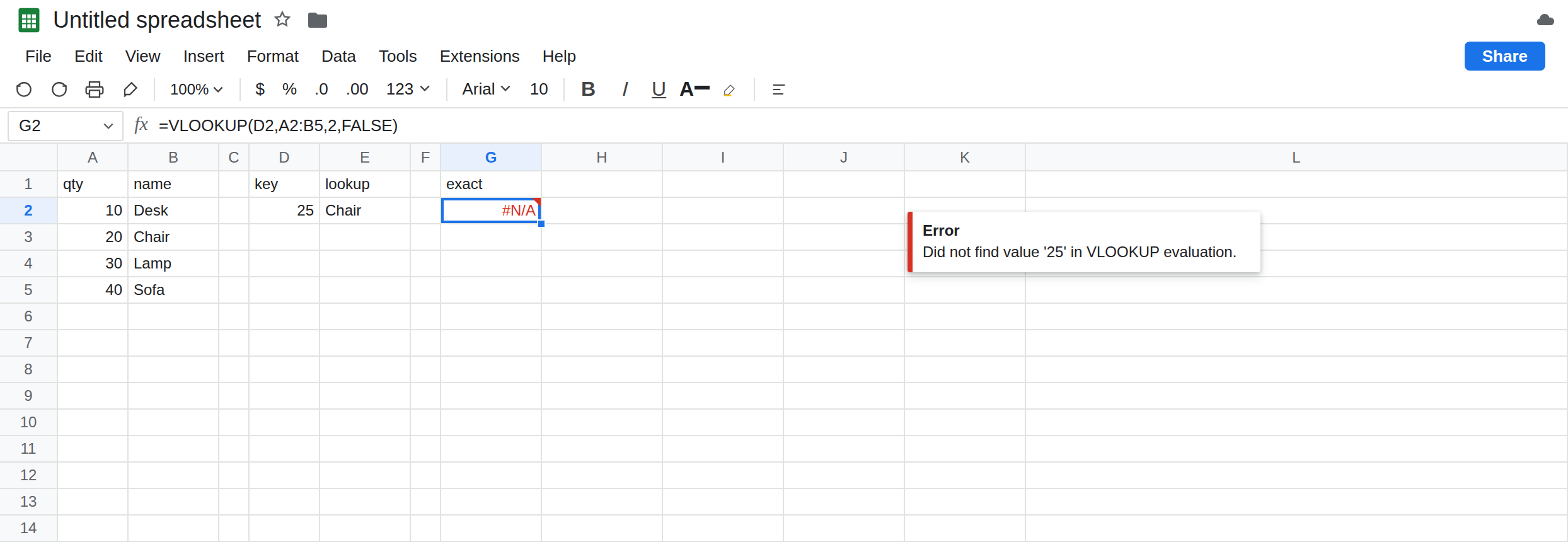
Exact functions disagree about 25. In G2 enter =VLOOKUP(D2,A2:B5,2,FALSE). G2 is #N/A. 25 is not a qty. In G3 enter =XLOOKUP(D2,A2:A5,B2:B5). G3 is #N/A. Default XLOOKUP is exact. E2’s Chair and G2’s #N/A are the same key. Leave G2 broken so the silent LOOKUP has an exact witness.

Unsorted is not a guaranteed #N/A. In I2 40, J2 Sofa. I3 10, J3 Desk. I4 30, J4 Lamp. I5 20, J5 Chair. In L2 enter =LOOKUP(25,I2:I5,J2:J5). L2 returns a name from column J, or #N/A. Do not treat that name as the closest break. The function still assumes ascending order. The result you can defend is E2, and only because A2:A5 is sorted. Leave L2 unused as a price.

Array form. In E9 enter =LOOKUP(D2,A2:B5). One range. It has more rows than columns, so Sheets searches the first column and returns the last column. E9 is Chair, same as E2, on this tall range. If the range were wider than it is tall, the search would run across the first row instead, and you would get a value from the bottom row. Vector form is the three-argument call, which is E2. Do not drop the result range and assume the search direction stayed put. Leave E9 next to E2.

Leave E2 as Chair. Leave G2 as #N/A. Leave E7 as #N/A for the key 5.

What is actually wrong

• Vector LOOKUP is approximate, always. There is no fourth argument to switch it off. If you need #N/A when 25 is absent, this is the wrong function. G2 and G3 are the exact calls.
• “Next smaller” is the largest key that is less than or equal to the lookup, which requires ascending order. 25 falls between 20 and 30, so the answer is the 20 row, Chair. 100 falls after 40, so the answer is Sofa, not #N/A. People use that on purpose for quantity breaks. They use it by accident for skus.
• A key below the first sorted value is the #N/A case. E7 is real. It does not mean the function became exact. 6 would still be #N/A on this list. 10 would be Desk.
• Unsorted input does not become an exact match, and it does not reliably become #N/A. L2 is not a price. Sort the search vector, or stop using LOOKUP.
• Keep the result vector the same height as the search vector. Array form hides that pairing: more rows than columns searches down the first column and returns the last column.

This is not XLOOKUP last match. That -1 is a scan direction on exact duplicates. LOOKUP of a duplicate key in a sorted run returns the last of the run, which is another reason not to use it for “the first sku.”

This is not MATCH approx unsorted except as the same approximate idea on MATCH. E2 does not return a position. It returns the name.

Fix

Leave E2 as Chair for 25 if the breaks are intentional. Leave G2 as the exact #N/A. Leave L2 unsorted and unused.

Quantity breaks, sorted. Keep E2. Document the column as breaks: 25 pays the Chair price because the break at 20 is the one in force until 30. E6’s Sofa for 100 is the top break, which you want only if “anything above 40 still pays Sofa” is the rule. If 100 should be an error, LOOKUP will not say so.

Sku lookups. In G5 enter =XLOOKUP(25,A2:A5,B2:B5,"missing"). G5 is missing. 25 is not a qty on the list, and the exact function says so. For a key that exists, =XLOOKUP(20,A2:A5,B2:B5,"missing") is Chair. Use XLOOKUP #N/A when the missing value is the whole story.

If you keep LOOKUP, sort A2:A5 ascending and use three arguments. Do not switch to the array form on a wide range without checking which direction it searches.

Do not wrap E2 in IFERROR. Chair is not an error. See IFERROR vs IFNA.

If LOOKUP returns a neighbor of the key you typed, the key was not an exact hit and the vector is doing its approximate job. If you needed #N/A, switch to XLOOKUP or VLOOKUP with FALSE. If the search column is not sorted, the name in the cell is not a break price. If the key is below every sorted value, #N/A is expected.

25 vs 100 vs an exact miss

Sorted LOOKUP of 25 is Chair. LOOKUP of 100 is Sofa. LOOKUP of 5 is #N/A. VLOOKUP of 25 with FALSE is #N/A. Default XLOOKUP of 25 is #N/A. Unsorted LOOKUP is not a price.