

Fix WORKDAY / WORKDAY.INTL #NUM! in Google Sheets (bad start date or holiday list)
Updated
WORKDAY returns a date that is N working days after a start date, skipping Saturday/Sunday and an optional holiday list. WORKDAY.INTL does the same with a custom weekend. #NUM! means the start, the day count, a holiday serial, or the weekend code is outside what those functions will accept. The formula parsed. The calendar math cannot land.
This page is WORKDAY / WORKDAY.INTL #NUM!. It is not out of domain (SQRT(-1), LN(0), FACT(171)). It is not #VALUE! from text that is not a date (WORKDAY("soon",5)). Keep the Google Sheets UI in English.
Recreate it on a blank sheet
Section titled “Recreate it on a blank sheet”- Open a blank spreadsheet. In A1 type
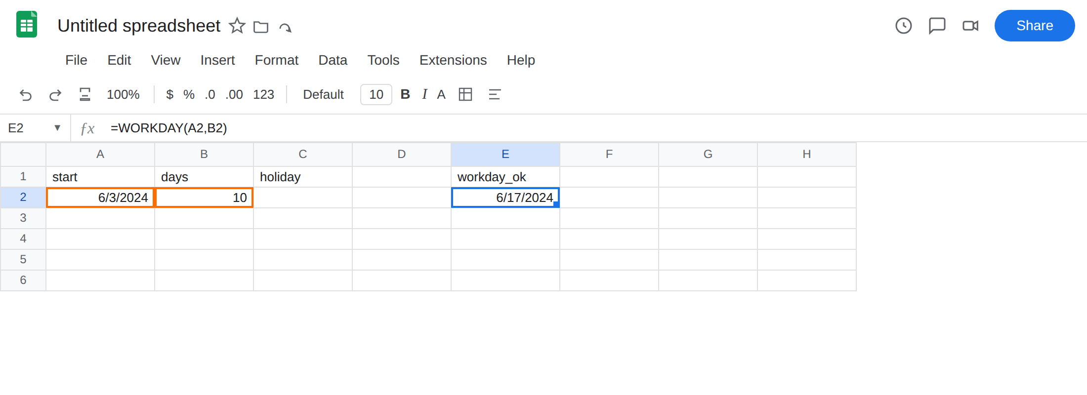
start. In A2 enter=DATE(2024,6,3)(a Monday). B1days. B210. C1holiday. - A date the function can return. In E1 type
workday_ok. In E2 enter=WORKDAY(A2,B2). The cell shows a date (17 June 2024 if there are no holidays). Format E2 as a date. That row is the control:WORKDAYworks on a real start and a modest day count.
- Invalid weekend code on WORKDAY.INTL. In E4 type
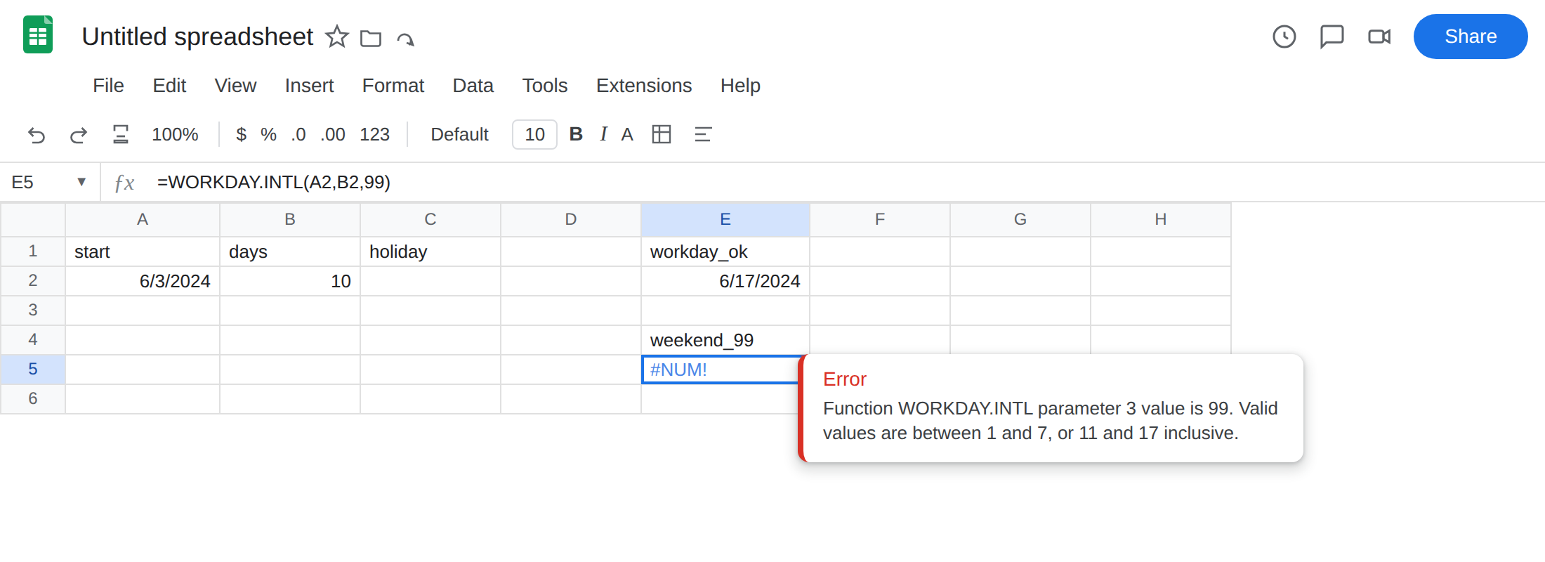
weekend_99. In E5 enter=WORKDAY.INTL(A2,B2,99). The cell shows#NUM!. Weekend must be1–7,11–17, or a seven-character0/1string (Monday-first).99is none of those. Leave E5 broken.
- Holiday list with an impossible serial. In C2 enter
=DATE(2024,6,19). In C3 type4000000as a number — not a date this calendar can use. In E7 typebad_holiday. In E8 enter=WORKDAY(A2,B2,C2:C3). The cell shows#NUM!. C2 is a fine holiday. C3 is not. Leave E8 broken.
Overflow days. In E11 enter =WORKDAY(A2,1000000). #NUM! — past the dates Sheets will return. Leave E11 broken.
Text start is a different error. =WORKDAY("kickoff",B2) is #VALUE!, not #NUM!. That is wrong type / DATEVALUE locale. Stay on E5 and E8 for this page.
Leave E5, E8, and E11 as the broken formulas. Leave E2 as the working date.
What is actually wrong
Section titled “What is actually wrong”WORKDAY.INTL’s third argument is a weekend code, not “how many weekend days.”1is Saturday+Sunday (theWORKDAYdefault).7is Friday+Saturday.11is Sunday only.99is not on the list.#NUM!.- A seven-character weekend string must be seven
0/1characters, Monday first (0000011is Saturday+Sunday)."weekend"and"11111111"are invalid. Sheets may show#NUM!or#VALUE!depending on the string. Treat both as a bad weekend argument. - Holidays must be valid date serials. A leftover
4000000, a negative serial Sheets will not use, or a value that is not a date in this file’s range, makesWORKDAY#NUM!. One bad cell inC2:C3poisons the call even when C2 is fine. - A huge
days(or a start already near the end of the calendar) asks for a date Sheets cannot represent. That is#NUM!, same family asFACT(171)overflow on out of domain — but the function here isWORKDAY, notFACT.
This is not SQRT of a negative. See out of domain. E5 parsed WORKDAY.INTL. Then the weekend code was rejected.
This is not #VALUE! from "kickoff" or 13/1/2024 as start text. G2 is that contrast. Parse the start with DATE / DATEVALUE first. Locale-shaped date text is DATEVALUE locale.
This is not #N/A. Nothing is being looked up. See what #N/A means.
Leave E5, E8, and E11 broken so #NUM! stays on the sheet.
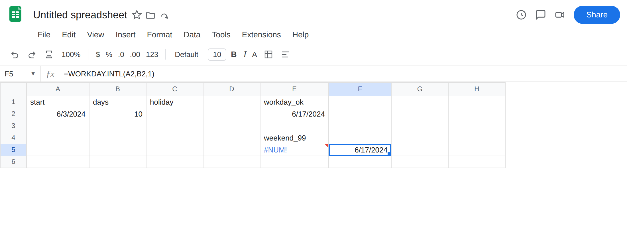
Pass a real weekend code. In F5 enter =WORKDAY.INTL(A2,B2,1). The cell matches E2. For Friday+Saturday, pass 7, or the string 0000110. Do not invent 99.
Clean the holiday list. Keep only real dates. In F8 enter =WORKDAY(A2,B2,C2). The cell is a date (C2 skipped as a holiday). Do not point holidays at a mixed column that still holds TBD or a huge number. Helper: =IF(ISNUMBER(C3),C3,"") and use a range of true dates only.
Shrink the day count. If you meant 10 workdays, use B2. Keep the start as =DATE(2024,6,3), not locale-fragile "6/3/2024".
Do not wrap E5 in IFERROR. You still have no end date. See IFERROR vs IFNA. IFNA will not catch #NUM!.
If WORKDAY / WORKDAY.INTL is #NUM!, read the weekend argument, then ISNUMBER on every holiday, then whether days is a realistic count. A text start is #VALUE! — different primer.
WORKDAY vs NETWORKDAYS
Section titled “WORKDAY vs NETWORKDAYS”WORKDAY answers “what date is 10 workdays after kickoff?” The result is a date.
NETWORKDAYS (and NETWORKDAYS.INTL) answers “how many workdays sit between these two dates?” The result is a count. Swapping them looks plausible in English and returns the wrong type of answer. #NUM! on NETWORKDAYS is a different domain (invalid dates in that pair). This page stays on WORKDAY / WORKDAY.INTL.
Do not replace WORKDAY with A2+B2 to dodge #NUM!. That adds calendar days, including Saturday and Sunday, and ignores holidays. Fix the weekend code or the holiday list. Keep the function that skips non-working days.