RANK.AVG and RANK.EQ score a tie differently

RANK.EQ(value, data, [is_ascending]) and RANK.AVG both rank a value inside a list. On a tie they disagree, and neither cell shows an error. RANK.EQ gives every tied value the best rank in the tie, then skips. Two scores tied for second are both rank 2, and the next score is 4. RANK.AVG gives the tie the average of the ranks it occupies. Those two scores are both 2.5. The next distinct score is still 4. RANK is RANK.EQ. A leaderboard that mixes the two functions will show 2 and 2.5 for the same person and look “off by half” with no triangle.

SORTN ties are a different spill. See SORTN ties mode. Keep the Google Sheets UI in English. Sheet Error is an independent formula-error library, not a Google product.

Recreate it on a blank sheet

1. Open a blank spreadsheet. In A1 type score. A2 10. A3 20. A4 20. A5 30. Four scores. 30 is the high score. 20 appears twice. 10 is alone at the bottom.

Descending, which is the default. Omit the third argument, or pass 0. Largest is rank 1. In C1 type eq. In C2 enter =RANK.EQ(A2,A$2:A$5). C2 is 4 (the 10). In C3 enter =RANK.EQ(A3,A$2:A$5). C3 is 2. In C4 enter =RANK.EQ(A4,A$2:A$5). C4 is 2. In C5 enter =RANK.EQ(A5,A$2:A$5). C5 is 1. The two 20s share rank 2. Nothing is rank 3. The 10 is rank 4.

AVG on the same list. In D1 type avg. In D2 enter =RANK.AVG(A2,A$2:A$5). D2 is 4. In D3 enter =RANK.AVG(A3,A$2:A$5). D3 is 2.5. In D4 enter =RANK.AVG(A4,A$2:A$5). D4 is 2.5. In D5 enter =RANK.AVG(A5,A$2:A$5). D5 is 1. The 30 and the 10 match RANK.EQ. Only the tie moved, from 2 to 2.5. The average of ranks 2 and 3 is 2.5. Both tied rows get that average. Rank 3 is still unused as a displayed rank.

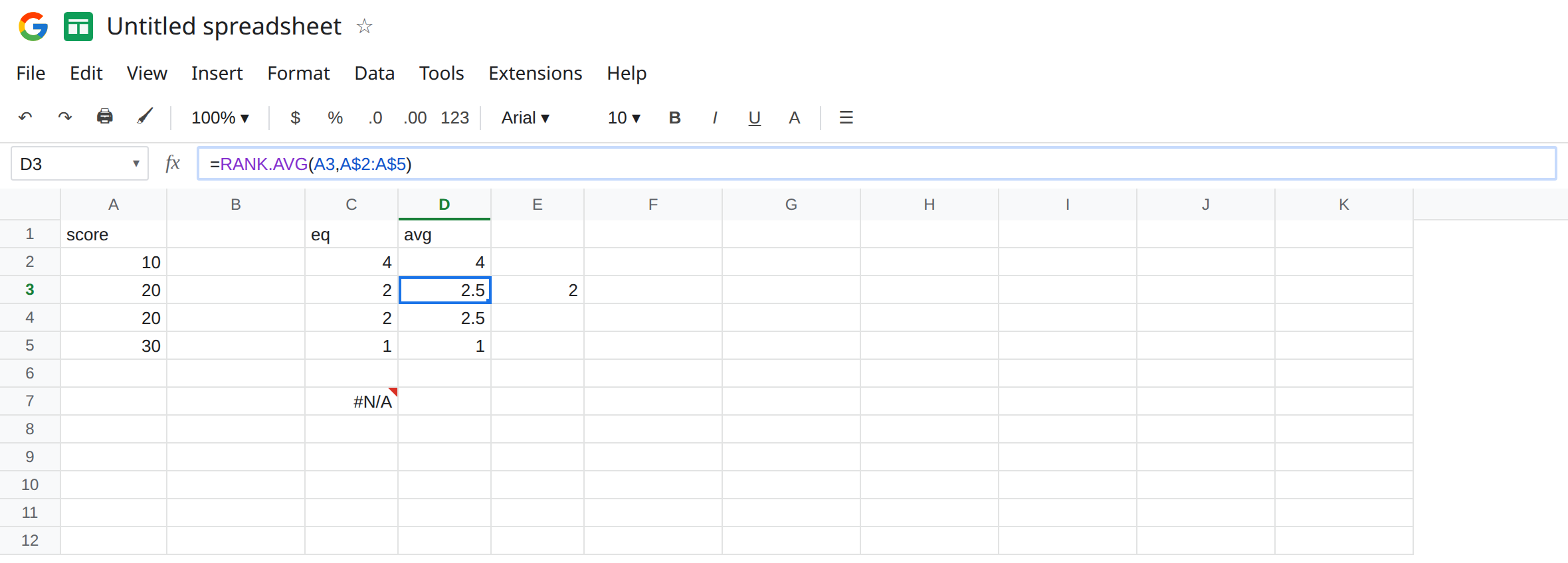
RANK is EQ. In E3 enter =RANK(A3,A$2:A$5). E3 is 2, the same as C3. If a sheet “switched to RANK” and the halves disappeared, it switched to RANK.EQ under the shorter name. It did not break RANK.AVG.

Ascending puts the small score first. Pass 1 as the third argument. In F5 enter =RANK.EQ(A5,A$2:A$5,1). F5 is 4. The high score 30 is last when the smallest value ranks first. C5, with the third argument omitted, is 1 for that same 30. In G3 enter =RANK.AVG(A3,A$2:A$5,1). G3 is 2.5. The tie still averages. Mixing a descending formula and an ascending formula in one standings column moves every rank and shows no triangle.

A value that is not in the list. In C7 enter =RANK.EQ(99,A2:A5). C7 is #N/A. The value has to occur in data. A typo in the value cell is #N/A, which is not the tie. Leave C7 broken. See what #N/A means only as the token. The tie in D3 is not #N/A.

Leave D3 as 2.5 and C3 as 2. Leave C7 as #N/A.

What is actually wrong

• Ties are the only place the two functions differ. Unique scores get the same rank from both, including the skipped number after a tie: the 10 is 4 either way, because one rank was consumed by the pair.
• RANK.EQ is competition ranking: share the best place, then skip. RANK.AVG is the average of the places the tie would have filled (2 and 3 → 2.5). Neither one assigns 2 and 3 to the two rows. If you need a unique rank per row, you need a second key (a timestamp, a name), not a different RANK suffix.
• The third argument defaults to descending (0). 1 is ascending. TRUE is not a documented substitute you should rely on in place of 1. Pass 0 or 1.
• The data range must be locked (A$2:A$5) when you fill down. =RANK.EQ(A3,A3:A6) slides the window and ranks 20 inside a different list. The rank changes with no tie involved. That is a relative-reference bug, the same shape as any filled formula.
• Text in the range is ignored. A header inside the range does not take a rank. A score stored as text does not compete, and RANK.EQ of that text value is #N/A or #VALUE! depending on the call. Keep scores numeric. =ISNUMBER(A3) should be TRUE.

This is not PERCENTILE.EXC #NUM!. See PERCENTILE.EXC bounds. Ranks here are ordinary numbers.

This is not SORT putting the rows in order. Rank numbers do not rearrange the sheet. The 30 stays in A5.

Fix

Leave C3 and D3 side by side so the tie stays visible. Leave C7 as #N/A.

Pick one function and use it on every row. If the board should say 2 and 2 with the next place 4, fill column C: =RANK.EQ(A2,A$2:A$5,0). If the board should split the places and show 2.5, fill column D: =RANK.AVG(A2,A$2:A$5,0). Do not mix C and D in one standings column.

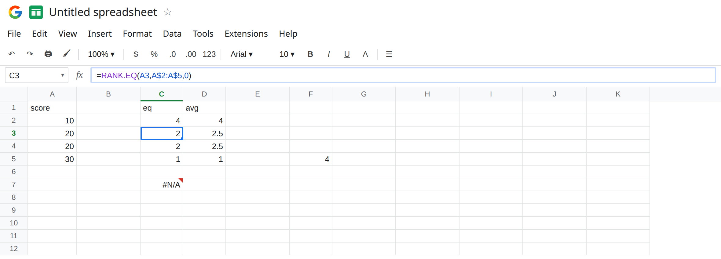
Pass the order on purpose. Add ,0 or ,1 instead of leaving a filled column half-omitted. F5 shows what 1 does to the high score.

A missing value is #N/A. Fix the value so it exists in the range, or switch to a lookup that has an if_not_found. Do not IFERROR the rank of 99 into 1. That person did not win.

If two rows show 2 and 2.5 for the same score, one formula is RANK.EQ (or RANK) and the other is RANK.AVG. If every rank shifted after you filled down, lock the data range. If the high score is rank 4, the third argument is 1.

The tie on this sheet

Score 30: both functions rank 1 (descending). Score 20 twice: RANK.EQ is 2 and 2, RANK.AVG is 2.5 and 2.5. Score 10: both rank 4. RANK matches the EQ column. There is no rank 3 in either column. C7’s #N/A is a value that is not in the list, not a tie.