

COUNTIFS of a date plus a text wildcard returns 0 when the types do not meet
Updated
COUNTIFS counts rows where every criterion matches. A date on the sheet is a serial number. The criterion ">=2024-01-01" is text, operator included, so it matches no serials. A wildcard such as ship* matches text and does not match a date serial. Put the quoted date on the date column, or put the wildcard on the date column by swapping the pairs, and the count is 0. There is no #VALUE! and no #N/A. The rows are visible. Fixing only one of the two pairs still leaves 0 if the other pair is aimed at the wrong type.
A single COUNTIF with a quoted date is COUNTIF date criteria. Dates stored as text, so a real date criterion skips them, are SUMIFS date text. A star you meant as a literal character is COUNTIF literal * ?. Keep the Google Sheets UI in English. Locale United States. Sheet Error is an independent formula-error library, not a Google product.
Recreate it on a blank sheet
Section titled “Recreate it on a blank sheet”- Open a blank spreadsheet. File → Settings → Locale → United States. Display language English. In A1 type
opened, B1status.
In A2 enter =DATE(2024,1,15). B2 shipped. In A3 enter =DATE(2024,2,1). B3 ship-hold. In A4 enter =DATE(2023,12,20). B4 shipped. In A5 enter =DATE(2024,3,1). B5 late. Format A2:A5 as a date if they show serials. All four are numbers. ISNUMBER(A2) is TRUE. Three dates fall in 2024. Two of those have a status that starts with ship (shipped and ship-hold). The count you want is 2. late is 2024 and does not start with ship. The December row starts with ship and is not 2024.
Both criteria, date written as text. In D1 type quoted. In D2 enter =COUNTIFS(A2:A5,">=2024-01-01",B2:B5,"ship*"). D2 is 0. The wildcard would have matched shipped and ship-hold. The date test never became a comparison of serials, so the AND fails on every row. Leave D2 as 0.
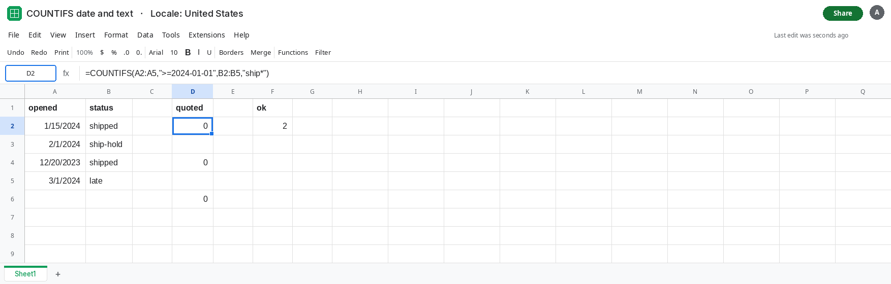
The wildcard on the date column. In D4 enter =COUNTIFS(A2:A5,"ship*",B2:B5,">="&DATE(2024,1,1)). The date test is now a real serial, and it is pointed at the status text. The wildcard is pointed at the date serials. D4 is 0. Each pair is the right idea on the wrong column. Leave D4 as 0.
One pair fixed, the other still quoted. In D6 enter =COUNTIFS(A2:A5,">="&DATE(2024,1,1),B2:B5,">=2024-01-01"). That second criterion is nonsense on a status column, and it is still text. D6 is 0. Building the date with DATE does nothing if you then compare it to shipped.
The control, both pairs typed for the column they face. In F1 type ok. In F2 enter =COUNTIFS(A2:A5,">="&DATE(2024,1,1),B2:B5,"ship*"). F2 is 2. January shipped and February ship-hold. December is out because of the year. March late is out because of the wildcard. Leave F2 as 2.
Leave D2 and D4 as 0.
What is actually wrong
Section titled “What is actually wrong”COUNTIFSAND-combines the pairs. One failed pair zeros the row. A quoted date fails every serial, so the wildcard never gets to save the count.- Wildcards apply to text. A date serial is a number.
ship*on column A matches nothing. A date comparison on column B matches nothing, becauseshippedis not a serial at or after 1 Jan 2024. - The operator belongs outside the date, joined with
&.">="&DATE(2024,1,1)is a criterion.">=2024-01-01"is a single string. The quotes in the first form cover only the operator. - Range length is not this zero. Mismatched range sizes are
#VALUE!. See COUNTIFS range size. D2’s ranges are the same height. The types inside them differ. - If the dates are text that only look like dates, the serial criterion is the one that returns
0, and the quoted string might accidentally match. CheckISNUMBERon A2 before you swap the criterion style. See SUMIFS date text and dates stored as text.
This is not COUNTIF date criteria alone. That page has one criterion. Here a second, text, criterion hides which pair is wrong if you only stare at the zero.
Leave D2 and D4 as 0. F2 is the pattern.
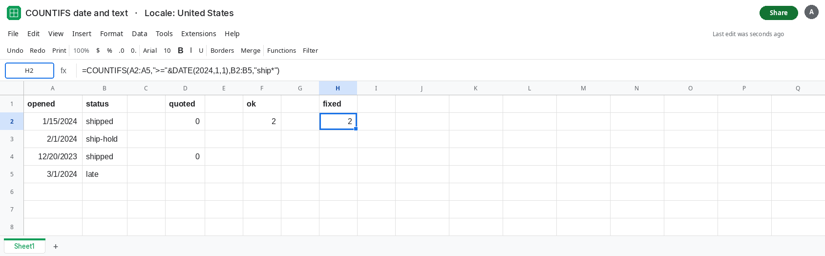
Point a serial date test at the date column and the wildcard at the text column. In H2 enter =COUNTIFS(A2:A5,">="&DATE(2024,1,1),B2:B5,"ship*"). H2 is 2. In H3 enter =COUNTIFS(A2:A5,">="&E2,B2:B5,"ship*") after you put =DATE(2024,1,1) in E2. H3 is 2 as well. The & joins the operator to a date value. The star stays on status.
Check each pair alone when the combination is 0. =COUNTIF(A2:A5,">="&DATE(2024,1,1)) is 3. =COUNTIF(B2:B5,"ship*") is 3 (two 2024 ship statuses plus December). The intersection is 2. If the date COUNTIF is already 0, you are still on the quoted-string problem or the cells are text. If the wildcard COUNTIF is 0, the star is on the wrong column or the statuses do not start with those letters. See COUNTIF literal * ? when the status itself contains a star you must match literally.
If D2 is 0 and F2 is 2, the quoted date was the failed pair. If both the quoted form and the DATE form are 0, look at which column received the wildcard. If the result is #VALUE!, the ranges are different sizes and this page is the wrong one.