Fix TOROW #REF! in Google Sheets when the horizontal spill is blocked

TOROW(array, [ignore], [scan_by_column]) flattens a block into one row. The spill moves right from the formula cell. A value in the next column, or anywhere in that width, stops the whole spill with #REF!. The tooltip names the occupied cell. Clearing cells under the formula does nothing, because TOROW does not write downward. That habit comes from TOCOL. Ignore codes make the row shorter. They do not change the direction.

This page is the horizontal spill. Ignore 2 and 3 hiding errors inside the stack are TOCOL ignore. The shared flatten primer is TOCOL / TOROW. Keep the Google Sheets UI in English.

Recreate it on a blank sheet

1. Open a blank spreadsheet. In A1 type sku. A2 101. A3 102. A4 103. Three skus in a column. You want them in a row.

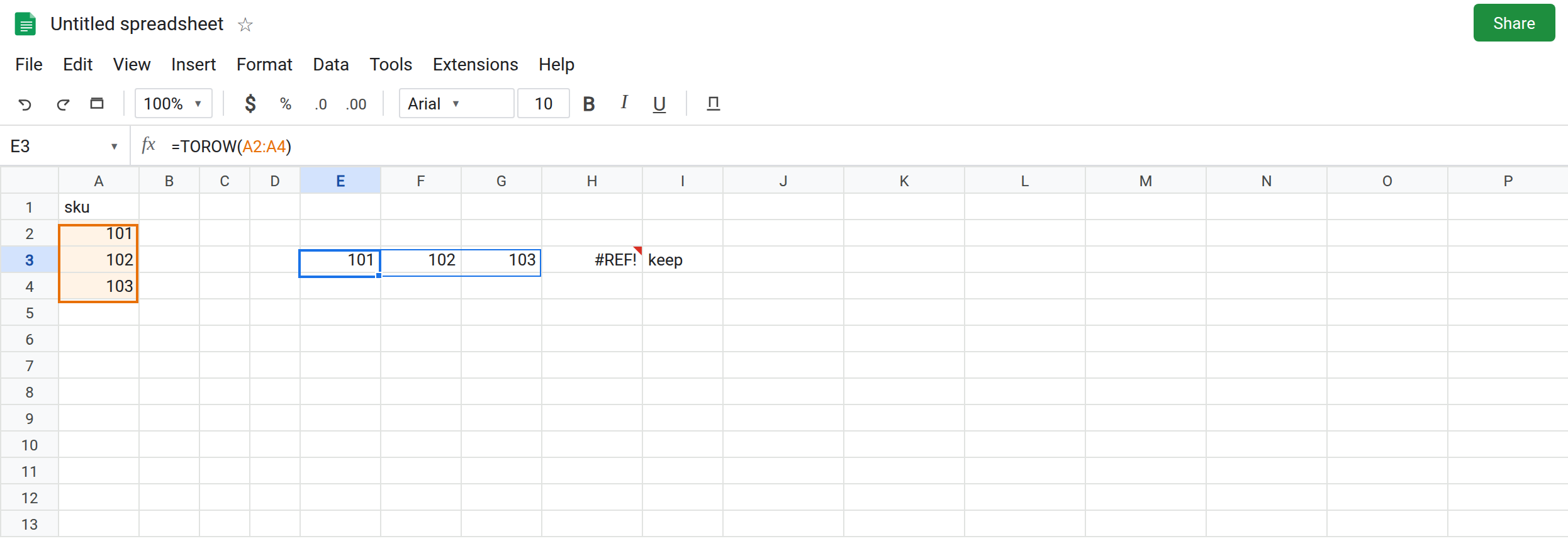
A clear row. In E1 type ok. Leave F1:G1 empty. In E1 you just typed a header, so put the formula on row 3 instead. In E3 enter =TOROW(A2:A4). The spill is E3 101, F3 102, G3 103. One row, three columns. That row is the control. TOCOL of the same range would have spilled down and looked identical to A2:A4. This one moved sideways.

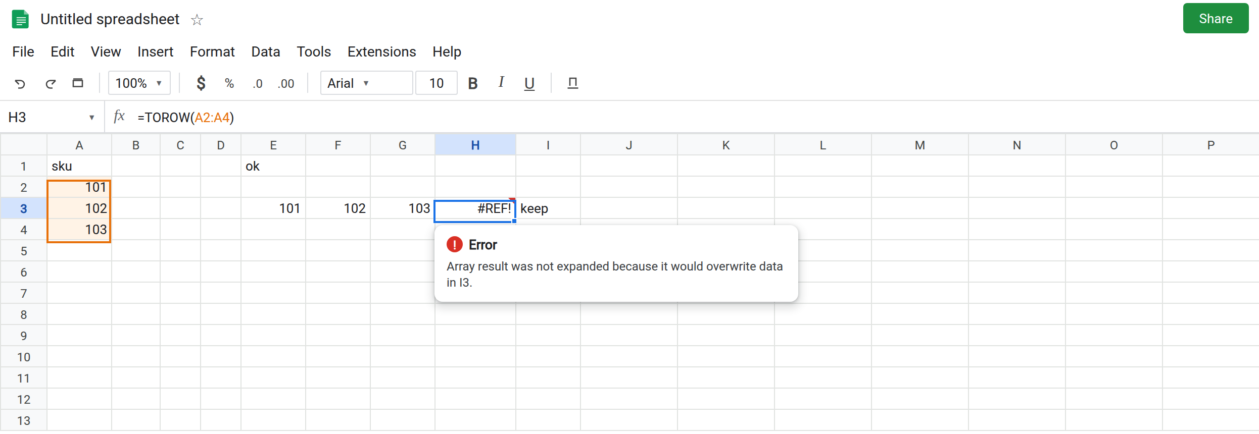
Blocked on the right. In I3 type keep. Leave H3 empty. In H3 enter =TOROW(A2:A4). The row needs H3:J3. I3 is occupied. H3 shows #REF!. The tooltip is Array result was not expanded because it would overwrite data in I3. Leave H3 broken.

A cell below does not block TOROW. In E4 type under. E3 is still 101, 102, 103. under sits beneath the first spilled cell and the row is fine. Delete under only if you want the grid tidy. It was not the #REF!. If this formula had been TOCOL, a value in E4 would have blocked it. The direction is the difference.

A wide block is a long row. In A6 type a, B6 b. A7 1, B7 2. In E6 enter =TOROW(A6:B7) on a clear stretch (move it if E6:H6 is not empty). Four cells across: a, b, 1, 2. Default scan is by row. In E8 enter =TOROW(A6:B7,0,TRUE) on a clear row. Scan by column: a, 1, b, 2. Same width, four columns. The third argument did not make a column. Leave both rows if the space is free so the order is visible.

Ignore shortens, then still goes right. Leave B2 empty. In A2 you have 101. Put a blank in a copy rather than destroying the control: in A10 type 101, leave B10 empty, A11 102. In E10 enter =TOROW(A10:B11,1). Ignore 1 drops the blank. The spill is three cells, not four: 101, 102, and whatever else remains in the block. It is still a row. If F10 is occupied, E10 is #REF! even though ignore made the row shorter. The shorter row might now fit. That is a size change, not a direction change.

TOCOL contrast. In K1 type down. Leave K2:K4 empty. In K2 enter =TOCOL(A2:A4). The spill goes down. A value in L2 would not block K2. A value in K3 would. Leave K2 as that column.

Leave H3 broken. Leave E3 as 101, 102, 103.

What is actually wrong

• TOROW’s result height is 1. Its width is the number of values that survive ignore. Three skus need the formula cell plus two cells to the right. I3 is inside that width. H3.
• Cells below the formula are outside the spill. E4. Clearing them is the TOCOL fix applied to the wrong axis.
• Ignore 0 through 3 match TOCOL. They change how many columns you need. They never spill downward. A remaining #N/A in the row means ignore was 0 or 1. See TOCOL ignore.
• scan_by_column reorders the row. TRUE on a grid reads down each column first. The output is still one row, so a blocker still sits to the right.
• A sheet that ends before the row finishes is also #REF!. Three values starting in the last column have nowhere to go. Move left. Do not shrink the source unless you meant to drop values.
• TRANSPOSE(TOCOL(...)) is a column turned sideways. It has the same width problem. If you already have a working TOCOL, TRANSPOSE is optional. TOROW is the direct function.

This is not HSTACK of uneven columns. See HSTACK row pad. H3’s tooltip names an overwrite, not a pad #N/A.

This is not a deleted reference. See after you delete. H3 still says TOROW.

Fix

Leave H3 broken.

Start where the row fits. Keep E3: =TOROW(A2:A4) with F3 and G3 empty. Or delete I3 and use the same formula in H3.

Need a column? Use K2: =TOCOL(A2:A4). Do not clear the row to the right and hope TOROW turns downward.

Shorter on purpose. =TOROW(A10:B11,1) after you have decided blanks should not take a column. Count the remaining values and reserve that many cells to the right before you enter the formula.

Do not wrap H3 in IFERROR. The three skus never appear, and I3 looks like a successful neighbor. See IFERROR vs IFNA.

If TOROW is #REF!, read the cell named in the tooltip. It is to the right, or inside the width of the row. A value underneath is not the blocker. If the row is simply in the wrong direction, you wanted TOCOL.