COUNTIF treats * ? and ~ as wildcards when you wanted the literal sku

COUNTIF(range, criterion) treats * as “any characters,” ? as “one character,” and ~ as the escape. A sku that really contains a star, written as the criterion N12*, counts N12, N120, and N12*. The total is quiet. There is no #N/A and no #VALUE!. The count is simply larger than the one row you meant.

This page is COUNTIF criteria, not a returned bay. VLOOKUP wildcards are VLOOKUP wildcards. XLOOKUP only wildcards in match_mode 2. See XLOOKUP match_mode.

Recreate it on a blank sheet

1. Open a blank spreadsheet. Keep the Google Sheets UI in English. In A1 type sku. A2 N12. A3 N120. A4 N12*. A5 N1. A6 n12. A4 is the four characters N, 1, 2, and a star. A6 is the same letters as A2 in lowercase.

The pattern you did not mean. In C1 type star_open. In C2 enter =COUNTIF(A2:A6,"N12*"). The cell shows 4. Counted: N12, N120, N12*, and n12. Not counted: N1. * may be empty, so N12 matches N12 followed by nothing. COUNTIF is not case-sensitive, so n12 matches too. You wanted the one star sku. You counted four rows.

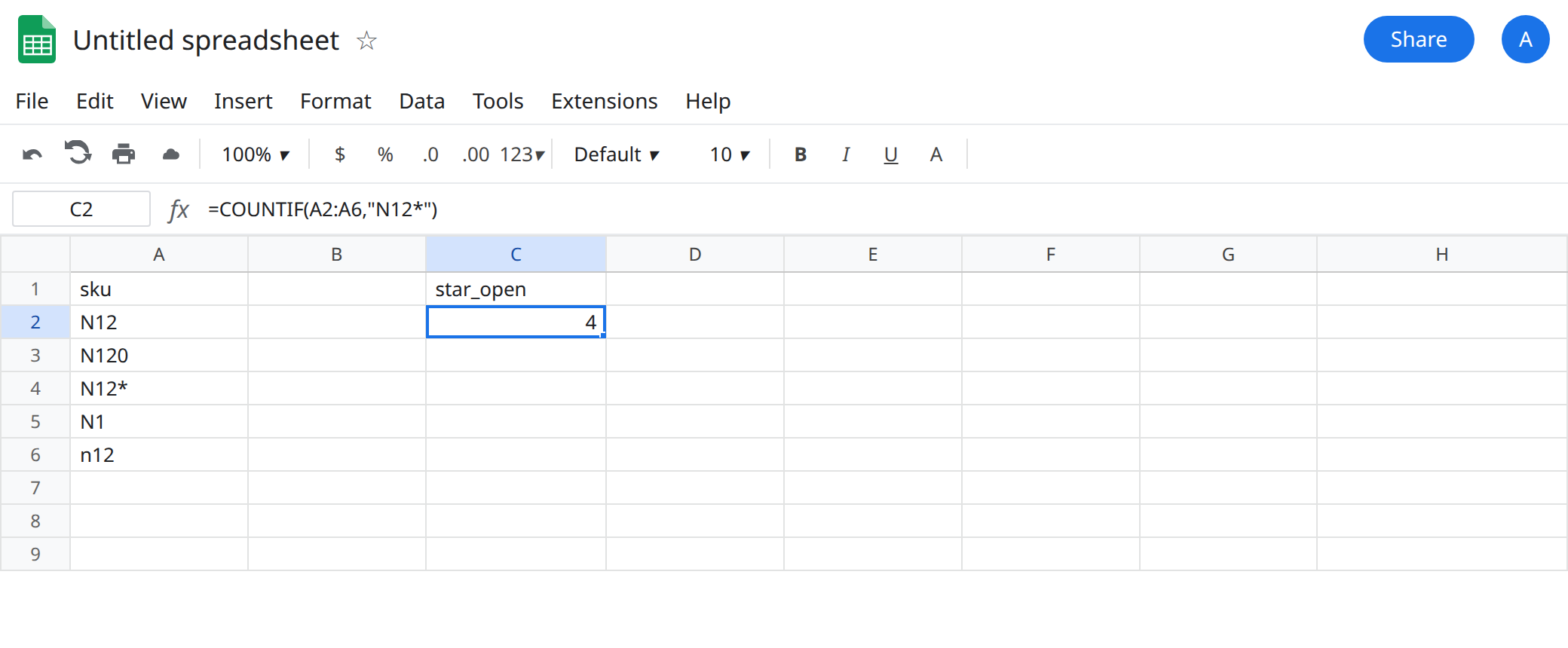
Question mark. In C4 type one_char. In C5 enter =COUNTIF(A2:A6,"N1?"). The cell shows 2: N12 and n12. ? is exactly one character. N120 has more than one character after N1. N12* has two characters after N1 (2 and *). N1 has zero.

Literal star. In C7 type literal. In C8 enter =COUNTIF(A2:A6,"N12~*"). The cell shows 1. Only A4. The tilde escapes the star that follows it.

Criterion sitting in a cell. In E1 type wanted. In E2 type N12*. In E4 enter =COUNTIF(A2:A6,E2). The cell shows 4, same as C2. Putting the star in a cell does not turn it into a literal. COUNTIF reads the text and still sees a wildcard.

A tilde that is part of the sku. In A8 type N12~. In C10 enter =COUNTIF(A2:A8,"N12~~"). The cell shows 1. A single ~ in the criterion escapes the next character. To find a tilde, you double it.

Leave C2 and E4 as 4. They are the bug. Leave C8 as 1.

What is actually wrong

• In a COUNTIF criterion, * is not an asterisk character until you escape it. It is “zero or more of anything.” N12* is a prefix test. The star sku is one of the rows that pass, which is why the count feels almost right and is still high.
• ? is one character, not “optional” and not “a question mark.” A sku that contains ? needs ~? the same way a star needs ~*.
• ~ escapes the next wildcard. ~* is a star. ~? is a question mark. ~~ is a tilde. A criterion that ends with a bare ~ is easy to misread; the escape applies to whatever character follows.
• The match is case-insensitive. n12 counts with N12 under N12*. If you needed case, COUNTIF is the wrong tool. EXACT inside SUMPRODUCT or FILTER is a different formula. Do not “fix” case by adding a tilde.
• A criterion cell is not a literal mode. E4 proves it. People store the sku in E2 so they can edit one cell, then the star starts matching the whole family.
• COUNTIFS uses the same wildcard rules on every text criterion. A numeric criterion does not. This page’s keys are text.

There is no error to catch. IFERROR around C2 returns 4. See IFERROR vs IFNA. The sheet is not failing. The pattern is wider than the sku.

COUNTIFS does not turn the star off when you add another condition. =COUNTIFS(A2:A6,"N12*",B2:B6,">0") still treats N12* as a prefix. Escape the text criterion and leave the numeric one alone. A numeric criterion never needs ~. If the second range is shorter than the first, you are on a size error, not a wildcard. The count in C2 is a full-height range of five sku cells, and the only surprise is which of them matched.

This is not approximate MATCH. See MATCH approx unsorted. MATCH type 0 also honors * and ?. Escaping is the same tilde. The value MATCH returns is a position, not a count.

Fix

Leave C2 and E4 broken so the unescaped count stays on the sheet.

Escape a fixed literal. Keep C8: =COUNTIF(A2:A6,"N12~*"). For a question-mark sku, =COUNTIF(A2:A6,"N12~?").

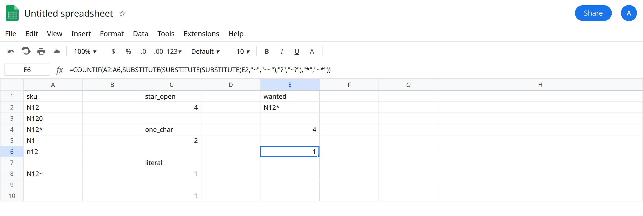
Escape a sku that lives in a cell. The cell may contain *, ?, or ~, so escape ~ first. In E6 enter:

=COUNTIF(A2:A6,SUBSTITUTE(SUBSTITUTE(SUBSTITUTE(E2,"~","~~"),"?","~?"),"*","~*"))

E2 is N12*. E6 shows 1. If you substitute * before ~, a tilde you just inserted gets escaped again and the count moves. Order is tilde, then question mark, then star.

You wanted the prefix. Then C2 is the right formula and the label should say “N12 and anything after it,” not “sku N12*.” Do not escape it.

Count one exact sku without learning wildcards. =SUMPRODUCT(--(A2:A6=E2)) compares with = and does not treat * as a pattern. That count is 1 for the star sku. It is also case-sensitive, unlike COUNTIF, so n12 will not ride along. Use it when the criterion must be literal and case must matter. Use escaped COUNTIF when you want COUNTIF’s case folding and a literal star.

If the count is bigger than the rows you can see with that exact text, the criterion still contains an unescaped * or ?.