

Dates stored as text sort wrong and break XLOOKUP and MATCH
Updated
A date can look like a date and still be text. It sits on the left of the cell. ISTEXT is TRUE. ISDATE is FALSE. Sort A → Z orders the characters, so 10/1/2024 can land before 2/1/2024. XLOOKUP and MATCH against a real date serial return #N/A. The day is on the sheet. The types are not equal.
SUMIFS skipping the same cells is SUMIFS date text. Turning the text into a serial is TO_DATE and DATEVALUE locale. A csv sku that is text is CSV text vs number. Keep the Google Sheets UI in English. File → Settings → Locale → United States for this recreate, so a real 3/4/2024 is 4 March.
Recreate it on a blank sheet
Section titled “Recreate it on a blank sheet”- Open a blank spreadsheet. In A1 type
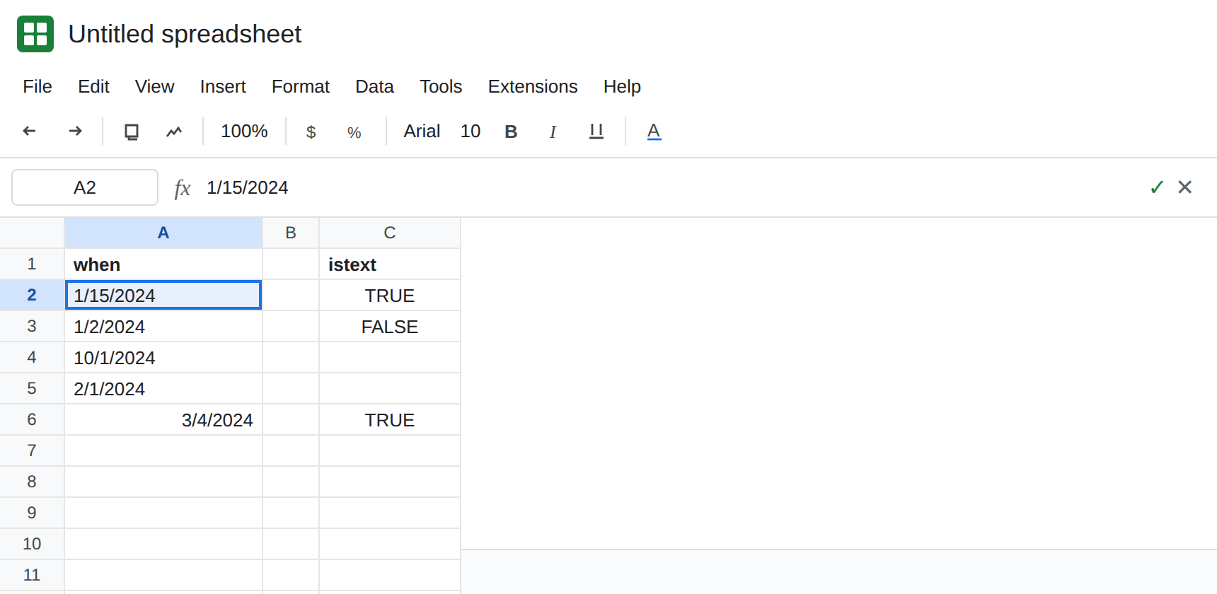
when. In A2 type an apostrophe and then1/15/2024. In A3 type an apostrophe and then1/2/2024. In A4 type an apostrophe and then10/1/2024. In A5 type an apostrophe and then2/1/2024. All four sit on the left. In A6 type3/4/2024without an apostrophe so Sheets stores a real date, right-aligned or centered as a date.
They are text. In C1 type istext. In C2 enter =ISTEXT(A2). C2 is TRUE. In C3 enter =ISDATE(A2). C3 is FALSE. In C6 enter =ISDATE(A6). C6 is TRUE. A6 is the control: a real date on the same sheet.
Sort A → Z is not calendar order. Select A1:A5. Data → Sort range → Sort range by column A (A to Z). If Sheets asks about a header, say row 1 is a header. The text rows come out in character order: 1/15/2024, then 1/2/2024, then 10/1/2024, then 2/1/2024. January 15 before January 2, and October before February. Nothing is #N/A. The sort did what text sort does. A6 stays a real date because it was outside the range. Put the four text dates back in A2:A5 in the order you first typed if you want the lookup below to match the paragraph. Or leave them sorted. The lookup does not care about row order.
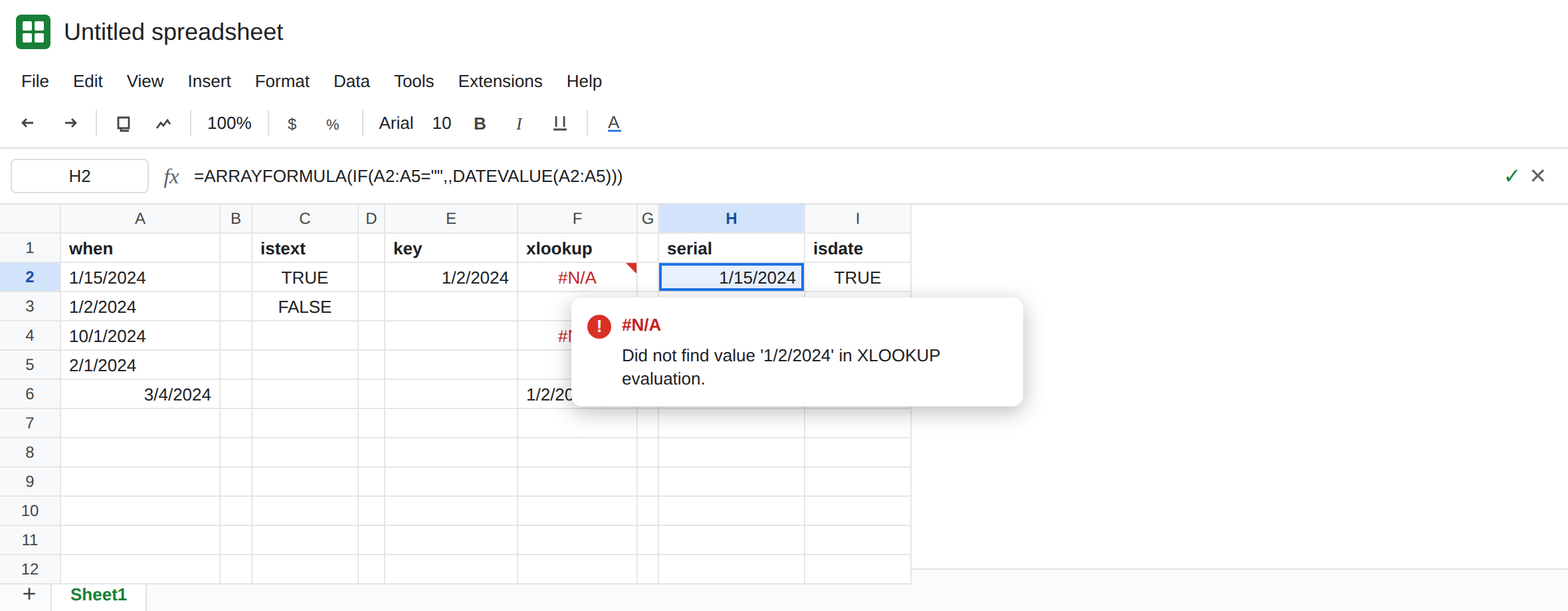
XLOOKUP misses the serial. In E1 type key. In E2 enter =DATE(2024,1,2). That is 2 January 2024, the same day A3 shows. In F1 type xlookup. In F2 enter =XLOOKUP(E2,A2:A5,A2:A5). F2 is #N/A. Tooltip: Did not find value in XLOOKUP evaluation. The day is visible in A3. The key is a serial and A3 is text. Leave F2 broken.
MATCH misses the same way. In F4 enter =MATCH(E2,A2:A5,0). F4 is #N/A. Exact match does not coerce text to a date. Leave F4 broken.
A text key hits. In F6 enter =XLOOKUP("1/2/2024",A2:A5,A2:A5). F6 returns the text 1/2/2024. Same column. The key type matches. That row is why the column looks “fine” until a real date searches it.
What is actually wrong
Section titled “What is actually wrong”- An apostrophe, a csv import, or a download that never parsed can store
1/2/2024as characters. Alignment is the hint.ISTEXT/ISDATEis the check. A format painted on the cell (Format → Number → Date) does not convert text. The serial never appears. - Sort A → Z compares character codes.
1equals1, then5versus2puts January 15 first.1versus2puts10/1/2024before2/1/2024. Calendar order needs date serials. XLOOKUPandMATCHwith match type0require an equal value. A serial is not equal to the characters1/2/2024. The#N/Ais a real miss. See XLOOKUP no match.if_not_foundwill hide it and still will not find the row.SUMIFSandCOUNTIFSskip the same cells without a triangle. The total is just short. That recreate is SUMIFS date text.- Locale decides how a real typed date is read. It does not reinterpret an apostrophe-forced string. See DATEVALUE day order.
Leave F2 and F4 as #N/A until the column is actually dates, so the miss stays visible.
Turn the text into serials, then sort. If the strings are month/day/year in this United States locale, in H2 enter =ARRAYFORMULA(IF(A2:A5="",,DATEVALUE(A2:A5))) and format H2:H5 as dates. H2:H5 are serials. ISDATE on H2 is TRUE. Sort that column, or paste values over A2:A5 after you have checked 2 January is 2 January and not 1 February. DATEVALUE follows locale. A day-first string on a United States sheet becomes the wrong serial or #VALUE!. See DATEVALUE locale.
Look up with the same type. After A2:A5 are serials, F2 finds 2 January. While they are text, search with the text key, as F6 does, and do not point DATE at that column.
Do not sort the text column and call it chronological. Data → Sort range will keep using character order until the values are dates. A custom display format will not change that.
If the days are left-aligned, ISTEXT is true, and XLOOKUP of a DATE is #N/A, convert the column. If ISDATE is already true and the lookup still fails, you are on spaces, types of the key, or a real missing day — not this page.