

FIXED returns text, so SUM stays 0 until you wrap VALUE
Updated
FIXED(number, [decimals], [no_commas]) rounds a number and returns text. FIXED(1234.5, 2) on a United States sheet is the string 1,234.50, not the number 1234.5. It is left-aligned if the column format is not forcing right. ISNUMBER is FALSE. SUM of text is 0, so a column of FIXED results looks rounded and adds to nothing. + 1 on that string is #VALUE!. Wrapping VALUE turns the string back into a number this locale can read.
ROUND returns a number. That is a different function, and binary residue on a scaled round is ROUND binary. Parsing locale-shaped text is VALUE() locale. Keep the Google Sheets UI in English. Locale United States. Sheet Error is an independent formula-error library, not a Google product.
Recreate it on a blank sheet
Section titled “Recreate it on a blank sheet”- Open a blank spreadsheet. File → Settings → Locale → United States. Display language English. In A1 type
n. A2 type1234.5. A3 type10. A4 type2.2.
FIXED looks like money and is text. In C1 type fixed. In C2 enter =FIXED(A2,2). C2 displays 1,234.50. In D2 enter =ISNUMBER(C2). D2 is FALSE. In D3 enter =ISTEXT(C2). D3 is TRUE. Fill C3 and C4 with =FIXED(A3,2) and =FIXED(A4,2). They display 10.00 and 2.20. The comma in C2 is a character in the string, inserted because the third argument default includes thousands separators.
SUM ignores the strings. In F1 type sum. In F2 enter =SUM(C2:C4). F2 is 0. The three rounded amounts are on the sheet. SUM does not add text. There is no #VALUE! on F2. Leave F2 as 0. That quiet zero is the bug people report as “FIXED will not total.”
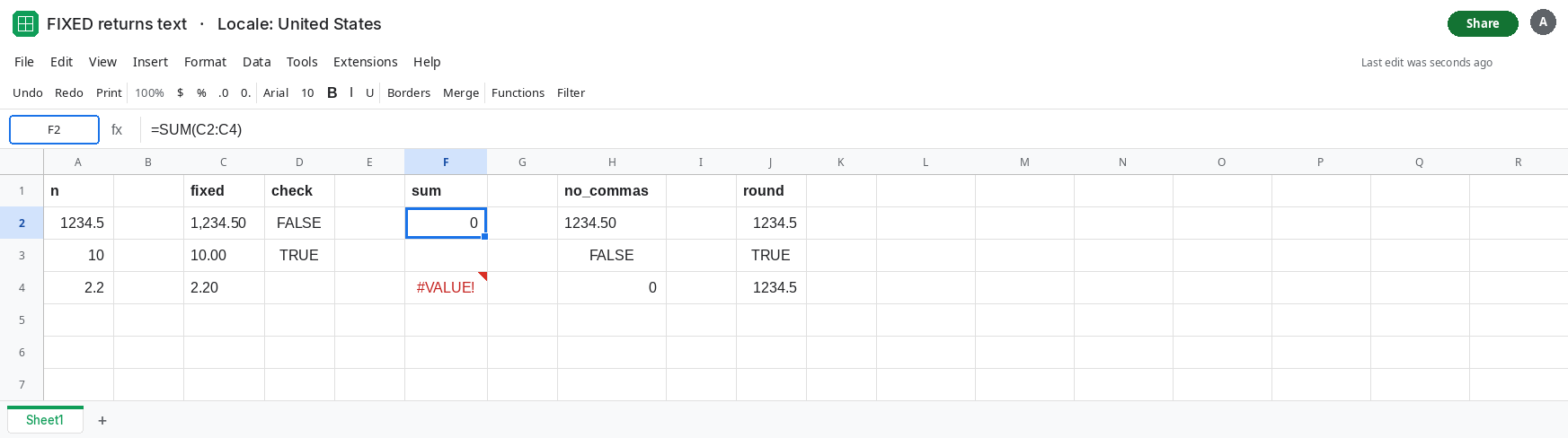
Addition is #VALUE!. In F4 enter =C2+1. F4 is #VALUE!. The tooltip expects a number. SUM skipped the text. The + operator does not. Leave F4 broken.
no_commas still returns text. In H2 enter =FIXED(A2,2,TRUE). H2 displays 1234.50 with no comma. In H3 enter =ISNUMBER(H2). H3 is FALSE. In H4 enter =SUM(H2). H4 is 0. The third argument only suppresses the thousands separator. It does not change the return type. Leave H4 as 0.
ROUND is the numeric control. In J2 enter =ROUND(A2,2). J2 is the number 1234.5 (format it as 0.00 if you want 1234.50 to display). In J3 enter =ISNUMBER(J2). J3 is TRUE. In J4 enter =SUM(J2). J4 is 1234.5. Same rounding request, a number back, and SUM works.
Leave F2 as 0 and F4 as #VALUE!.
What is actually wrong
Section titled “What is actually wrong”FIXEDis a text function that happens to round. The decimals argument chooses how many digits land in the string. The result is text even when every character is a digit.SUMskips text. A total of0with no triangle means the range held no numbers. It does not mean the rounded values were zero. CheckISNUMBERon oneFIXEDcell.- Arithmetic operators do not skip text.
C2+1is#VALUE!. That is wrong type after a successfulFIXED, not a failure insideFIXEDitself. - The default thousands separator follows the locale. On United States the string contains commas.
VALUEcan parse that string here. On a locale that does not treat,as thousands,VALUEof the sameFIXEDstring is#VALUE!. See VALUE() locale. Passing TRUE forno_commasavoids the separator and still leaves text. - Number format on C2 does not convert the string. The formula bar still shows
FIXED. Formatting is a display of a number you already have.ROUNDplus a format is that path.FIXEDis the other path.
This is not SUMIF text numbers, where the sum range contains imported digits with an apostrophe. Here the text was manufactured by FIXED.
Leave F2 as 0 and F4 as #VALUE!.
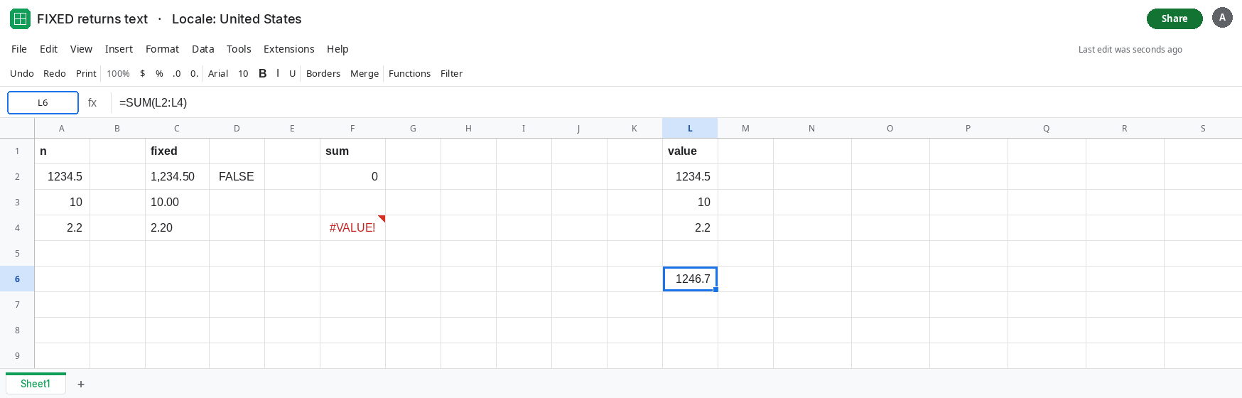
VALUE the string, on this locale. In L2 enter =VALUE(C2). L2 is 1234.5. Fill L2:L4 from the three FIXED cells, or use =ARRAYFORMULA(VALUE(C2:C4)). In L6 enter =SUM(L2:L4). L6 is 1246.7 (1234.5 + 10 + 2.2). The commas in C2 parsed because the locale is United States.
Or round as a number and format the cell. =ROUND(A2,2) in J2 is already the control. Select the result and use Format → Number if you need two decimals on screen. SUM of those cells counts them. You do not need FIXED unless a downstream step truly requires text, such as a label.
If VALUE of FIXED is #VALUE!, the thousands characters do not match the locale. Use =VALUE(FIXED(A2,2,TRUE)) so the string has no separator, then confirm ISNUMBER. See VALUE on percent text when the string also contains a currency symbol FIXED did not add.
If SUM of a FIXED column is 0 and ISTEXT is TRUE, the round worked and the type is text. If one cell of that column is #VALUE! under a +, you added text. If ISNUMBER is TRUE, the formula is ROUND or a later VALUE, and the total should move.