SEQUENCE treats 2024-01-01 as subtraction, so the series starts at 2022

SEQUENCE(rows, columns, start, step) will build a date series when start is a date serial and step is a number of days. Typed as 2024-01-01, with no quotes and no DATE, those characters are arithmetic. 2024 - 1 - 1 is 2022. The spill is 2022, 2023, 2024, 2025. Format them as dates and they are still those integers, not January 2024. The function did the subtraction you wrote.

A row count of 0 or a negative size is SEQUENCE size. A spill blocked by a neighbor is SEQUENCE spill. Keep the Google Sheets UI in English. Sheet Error is an independent formula-error library, not a Google product.

Recreate it on a blank sheet

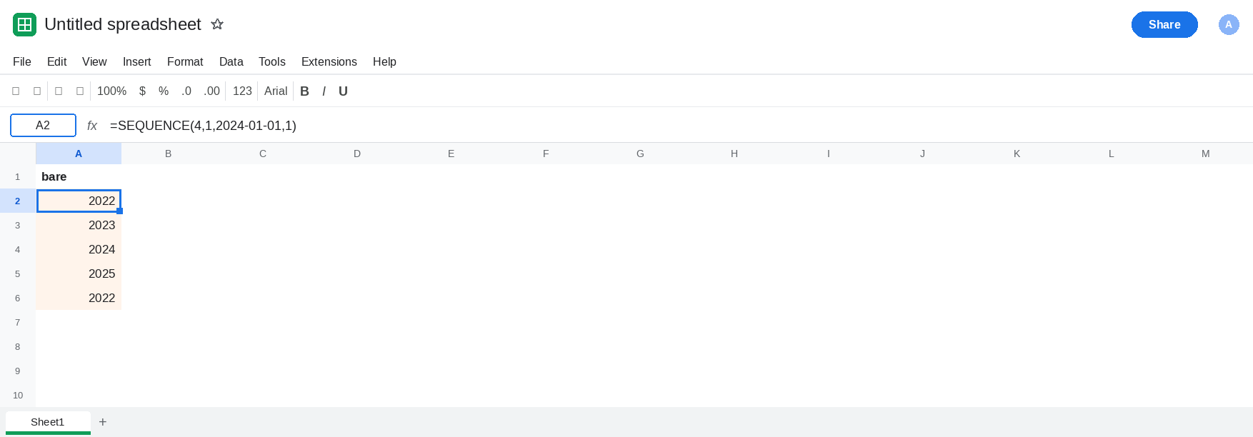
1. Open a blank spreadsheet. You do not need source data. In A1 type bare. In A2 enter =SEQUENCE(4,1,2024-01-01,1). The spill is 2022, 2023, 2024, 2025. In A6 enter =2024-01-01. A6 is 2022. That single cell is the start SEQUENCE received. Nothing in A2 parsed a calendar date. Leave A2 as those four integers.

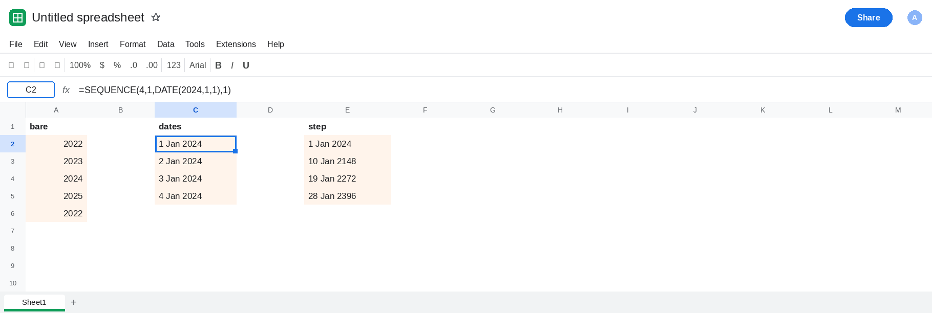
DATE as the start. In C1 type dates. In C2 enter =SEQUENCE(4,1,DATE(2024,1,1),1). The spill is four serials, one day apart. Select C2:C5 and choose Format → Number → Date. The cells show 1 Jan 2024 through 4 Jan 2024, in your locale’s date format. The step 1 is one day because a date serial counts days. Leave C2 formatted as dates. That block is the control.

A week. In C7 enter =SEQUENCE(4,1,DATE(2024,1,1),7). Format C7:C10 as dates. The cells are 1 Jan 2024, 8 Jan 2024, 15 Jan 2024, 22 Jan 2024. The step is the number 7, not a second date. Leave C7 as that weekly list.

A date in the step slot. In E1 type step. In E2 enter =SEQUENCE(4,1,DATE(2024,1,1),DATE(2024,1,8)). DATE(2024,1,8) is a serial on the order of forty-five thousand, not the number 7. The second row is more than a century after the first, not 8 Jan 2024. Format E2:E5 as dates and read them. Leave E2 as that jump. The weekly series is C7. E2 used the serial as a step.

A quoted string is not the repair. In E7 enter =SEQUENCE(4,1,"2024-01-01",1). Depending on locale, Sheets may coerce that text into a serial, or the cell may be #VALUE!. Either outcome is a coercion, not a date you wrote down. Do not keep E7 as the series you publish. The call you can defend is C2. Dates stored as text in ordinary cells are dates stored as text.

Leave A2 as 2022 and the three integers under it. Leave C2 as 1 Jan 2024. Leave E2 as the century-scale jump.

What is actually wrong

• Inside a formula, 2024-01-01 is subtraction. A6 proves the value is 2022 before SEQUENCE repeats it. Hyphens are minus signs. They are not date punctuation in that position.
• DATE(year, month, day) returns a serial. SEQUENCE then adds step for each next cell. Step 1 is the next day. Step 7 is the next week. C2 and C7.
• Putting DATE(2024,1,8) in the step argument adds that serial, not seven days. E2. The start and the step are different jobs. The end date does not belong in step.
• A quoted ISO string might coerce. E7. Locale and the cell’s format decide whether you see a date, a serial, or #VALUE!. DATEVALUE has its own locale failures. See DATEVALUE locale. Build the start with DATE.
• Formatting A2 as a date does not turn 2022 into 1 Jan 2024. It turns the number 2022 into a day in 1905. The value has to change. Format is how C2 becomes readable after the serial is correct.

A negative row count is #NUM! and never gets as far as the start. See SEQUENCE size.

Fix

Leave A2 as the subtraction so the bare expression stays visible.

Start from DATE, step in days. Keep C2 for a daily list. Keep C7 for a weekly list. In C12 enter =SEQUENCE(12,1,DATE(2024,1,1),1) and format the spill as dates when you need a year of days. Twelve rows, step 1, start 1 Jan 2024.

The gap between two dates is subtraction of serials, in the step only after you mean a day count. =DATE(2024,1,8)-DATE(2024,1,1) is 7. You may pass that as the step. You may not pass DATE(2024,1,8) itself and expect the same week.

Do not wrap A2 in TEXT to force a year to appear. TEXT(2022,"yyyy") is 1905, the year of serial 2022, which is a second wrong reading. See TO_DATE when a serial is already correct and only the format is general.

If a SEQUENCE of dates shows 2022, 2023, 2024, the start is an unquoted 2024-01-01 and the minuses already ran. Use DATE. If the second date is decades away, the step is a date serial. Use a day count. If the cell is #NUM! before any date appears, the row or column count is the size page.