

SUBTOTAL 9 and 109 do not treat hidden rows the same way
Updated
SUBTOTAL(function_code, range) aggregates a vertical range and skips rows a filter has hidden. It always skips those filtered rows, whether the code is 9 or 109. The 100 you add to the code is only about rows you hid yourself with Hide row. Code 9 is SUM and includes manually hidden rows. Code 109 is SUM and excludes them. Codes 1–11 include manual hides. Codes 101–111 exclude them. SUM includes everything. A dashboard that uses 9 because “we filtered” still counts a row someone hid by hand.
Keep the Google Sheets UI in English. Sheet Error is an independent formula-error library, not a Google product.
Recreate it on a blank sheet
Section titled “Recreate it on a blank sheet”- Open a blank spreadsheet. In A1 type
qty. A210. A320. A430. A540. The plain sum is100.
Both codes, nothing hidden. In C1 type code9. In C2 enter =SUBTOTAL(9,A2:A5). C2 is 100. In D1 type code109. In D2 enter =SUBTOTAL(109,A2:A5). D2 is 100. In E1 type sum. In E2 enter =SUM(A2:A5). E2 is 100. Three controls, all 100.
Hide a row by hand. Right-click the row header for row 4 (the 30) and choose Hide row. Row 4 disappears. C2 stays 100. Code 9 still sees the hidden 30. D2 becomes 70 (10+20+40). Code 109 skips the row you hid. E2 stays 100. SUM never cared. Leave row 4 hidden while you read those three cells.
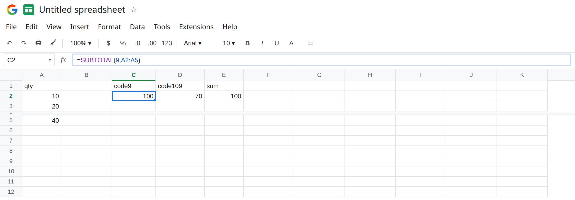
Unhide, then filter. Right-click a nearby row header and choose Unhide rows, or use the small arrow in the row headers, so row 4 is back. C2 and D2 are both 100 again.
Select A1:A5. Data → Create a filter. Click the filter icon in A1 and clear 40 only. Row 5 drops out of view because of the filter, not because you chose Hide row. C2 is 60. D2 is 60. E2 is still 100. Filtered-out rows leave both subtotals. They do not leave SUM. The 100 versus 101 split did nothing here. Both codes already skip filters.
Manual hide on top of a filter. With 40 still filtered out, hide row 4 again with Hide row. The visible numbers are 10 and 20. C2 is 60 (10+20+30: code 9 still includes the hand-hidden 30, and the filtered 40 is already gone). D2 is 30 (10+20 only). The filter and the manual hide are stacked. Unhide row 4 and turn the filter off (Data → Remove filter) before you call either cell wrong.
A code that is not a sum. =SUBTOTAL(1,A2:A5) is AVERAGE, including manual hides. 101 is AVERAGE ignoring them. 3 is COUNTA, 103 is COUNTA ignoring manual hides. The first digit you add is the “ignore manual hides” switch. It does not change SUM into COUNT.
Leave the sheet with the filter removed and row 4 hidden, so C2 is 100 and D2 is 70, if you want the manual-hide contrast left in place. Or leave the filter on and row 4 visible, so both codes are 60 and E2 is 100.
What is actually wrong
Section titled “What is actually wrong”- Filtered rows are out for every code. Choosing
109does not “turn filtering on.” Choosing9does not “turn filtering off.” - Manually hidden rows are in for
1–11and out for101–111. Hide row is not a filter. The menu path is different, and the codes treat it differently. SUM,COUNT,AVERAGE,MIN, andMAXignore neither filters nor manual hides. ReplacingSUBTOTALwithSUMto “simplify” freezes the total at100while the filter hides40.SUBTOTALignores otherSUBTOTALresults inside its range, so a subtotal placed in the column you are totaling is not added again.SUMwould add it. That is a second reason the two functions diverge, separate from hiding.- The function is built for vertical ranges. Hiding a column does not change
SUBTOTALof a row the way hiding a row changesSUBTOTALof a column. - Put the formula beside or above the table. A formula in A6 is inside the filter body the moment the filter range grows to include it, and the summary can vanish when that row is filtered out.
This is not FILTER the function, which spills matching rows and returns #N/A when nothing matches. See FILTER no match. The menu filter on this page hides rows in place.
This is not a #VALUE! from SUMIFS range size. See COUNTIFS range size. C2 and D2 are numbers.
Pick the code for the hide you actually use. For a filter menu, 9 and 109 match, and either is fine if nobody also uses Hide row. If people hide rows by hand and those rows should leave the total, use 109. If a hand-hidden row should stay in the total, use 9. In D2 keep =SUBTOTAL(109,A2:A5) when the 30 you hid should drop out.
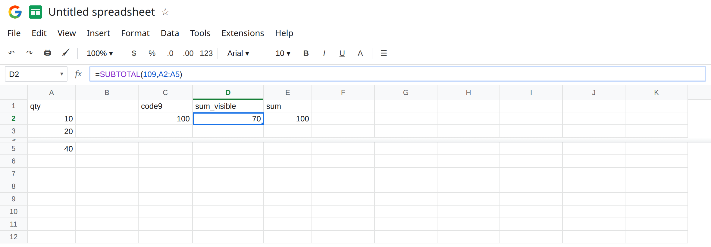
Label the header. sum_visible next to 109 is clearer than a bare 9. The same 100 switch applies to the other pairs: 1/101 AVERAGE, 2/102 COUNT, 3/103 COUNTA, 4/104 MAX, 5/105 MIN.
Do not wrap D2 in IFERROR. A change from 100 to 70 is the hide working. See IFERROR vs IFNA.
If 9 and 109 disagree, a row in the range is manually hidden. If they agree and SUM is larger, a filter is hiding rows (or both a filter and a manual hide are in a combination that happens to match). If all three agree, nothing is hidden. Unhide and remove the filter to get back to 100, then decide which code the sheet should keep.
Filter vs Hide row
Section titled “Filter vs Hide row”Filter off, row 4 hidden by hand: code 9 is 100, code 109 is 70, SUM is 100. Filter hiding 40, nothing else hidden: code 9 and code 109 are both 60, SUM is 100. The 100 added to the function code is the manual-hide switch only.