The first true conditional formatting rule is the one that paints

Conditional formatting rules on a range are a list. Google’s help states the order: rules are evaluated in the order listed, and the first rule that is true sets the format of the cell. Later rules do not get a turn on that cell. There is no second checkbox called stop if true. The list is that stop. A green rule under a red rule never paints a cell the red rule already matched. Drag the green rule above the red one when green is the format you wanted.

A formula that only fills the first column is CF formula range. A color scale on words is color scale on text. Keep the Google Sheets UI in English. Sheet Error is an independent formula-error library, not a Google product.

Recreate it on a blank sheet

1. Open a blank spreadsheet. In A1 type status, B1 hours. A2 open, B2 12. A3 open, B3 3. A4 shut, B4 12. You want open rows in green, and you also wrote a rule that paints any hours over 10 in red. A2 is both: open and 12.

The red rule first. Select A2:B4. Format → Conditional formatting. Single color. Format cells if Custom formula is. Formula: =$B2>10. Fill: red. The $ keeps the test on column B while the fill walks across the row. See CF formula range if only column A goes red. Done. A2:B2 and A4:B4 are red. A3 stays plain. 3 is not over 10.

The green rule under it. With the panel still open, Add another rule on A2:B4. Custom formula =$A2="open". Fill: green. Done. Look at the list. The red rule is above the green rule. A2 is still red. A2 is open, and the green formula is true, and the cell did not turn green. A3 is green, because the red rule is false there (3 is not over 10) and the green rule then runs. A4 stays red. shut is not open. Leave the list in this order.

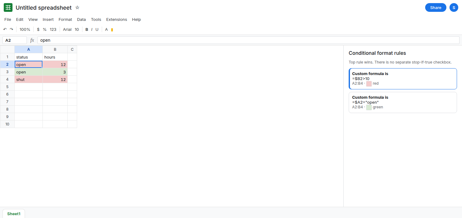
Reordering is the whole mechanism. Drag the green open rule above the red rule. A2 turns green. The red rule is still true for B2, and it no longer paints A2, because a true rule already won. A4 is still red: the green rule is false on shut, so the red rule runs. Drag the red rule back to the top and A2 is red again. Leave red on top so the blocked green rule stays visible.

A single-color rule and a color scale on the same cells follow this list too. The first true rule, or the first rule that applies, is the one you see. See color scale on text for a scale that never had a true category.

What is actually wrong

• The first true rule defines the format. “True” means that rule’s condition matched this cell. Both formulas match A2. Only the upper one paints. Adding a third rule under both does not create a blend.
• Sheets does not offer Excel’s stop-if-true flag as a separate control. You do not enable stopping. You change which rule is first. Dragging is the edit. The panel’s order is the order of evaluation, top to bottom.
• The apply-to range still matters. A green rule whose range is only A2:A4 will not paint B2 even after you drag it to the top. Read the range on the rule that “lost.” This recreate uses A2:B4 for both.
• Copy and paste can bring rules with the cells and stack duplicates. Two copies of the red rule on top of green keep A2 red. Delete the duplicate. The list is doing what it lists.

This is not data validation. A red fill does not block the typed 12. See reject versus warning.

Fix

Leave both rules on the sheet. Put the format you want for the overlap above the other.

Green wins on open, including open rows over 10. Drag =$A2="open" above =$B2>10. A2 is green. A3 is green. A4 is red, because it is not open and it is over 10.

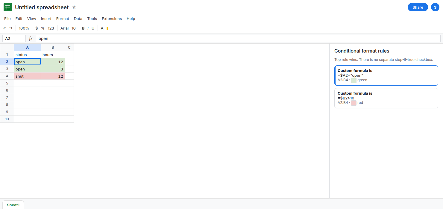
Red wins on large hours, including open ones. Drag =$B2>10 back to the top when a large hour should shout louder than the status color. A2 is red again. That is a choice of order, not a broken green formula.

One rule with both tests, when the overlap should be a third color. Custom formula =AND($A2="open",$B2>10) with its own fill, placed above the two broader rules, paints only A2. AND in a custom formula is a Sheets function. Inside QUERY it would be different. This is not a query string.

Do not wrap the custom formula in IFERROR. A formula that errors does not paint, and you would hide a #REF! in the rule. See IFERROR vs IFNA.

If a later rule never shows on a cell that meets its condition, a rule above it is already true. Drag them. If the cell is outside the later rule’s range, widen that range. The order cannot paint a cell the rule does not cover.