XLOOKUP match_mode: wildcard and next larger are not exact

XLOOKUP has six arguments. The fifth is match_mode: 0 exact (the default), 1 exact or next larger, -1 exact or next smaller, 2 wildcard (* and ?). The sixth is search_mode (first, last, or binary). A star in the key does nothing in mode 0. The same star in mode 2 matches a prefix. Mode -1 is not “search from the bottom.”

This page is match_mode. Last-match and binary search are XLOOKUP search_mode. An exact miss with if_not_found is XLOOKUP #N/A. VLOOKUP wildcards are VLOOKUP wildcards.

Recreate it on a blank sheet

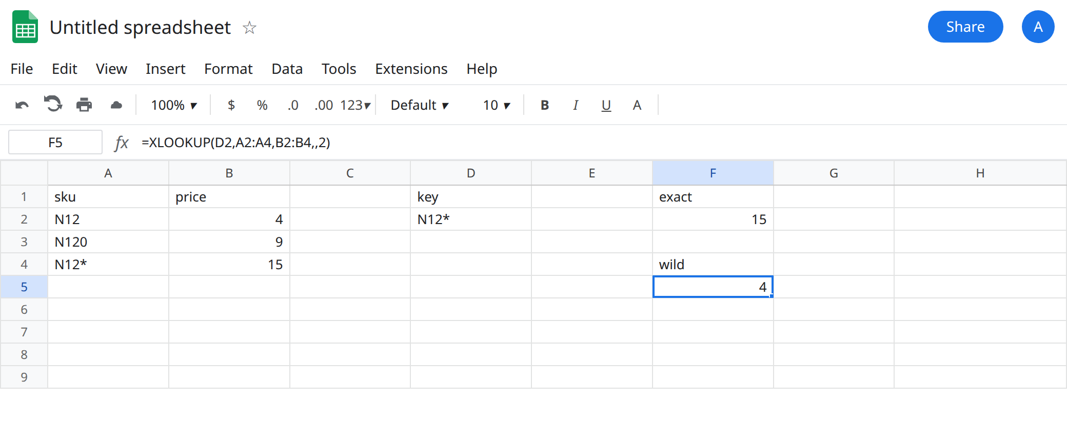
1. Open a blank spreadsheet. Keep the Google Sheets UI in English. In A1 type sku, B1 price. A2 N12, B2 4. A3 N120, B3 9. A4 N12*, B4 15. The fourth sku is the characters N, 1, 2, star. In D1 type key. D2 N12*.

Exact, the default. In F1 type exact. In F2 enter =XLOOKUP(D2,A2:A4,B2:B4). The cell shows 15. Mode 0 looks for the sku whose text is exactly N12*. The star is a character. N12 in A2 is not a match.

Wildcard mode. In F4 type wild. In F5 enter =XLOOKUP(D2,A2:A4,B2:B4,,2). The fifth argument is 2. if_not_found is omitted, so you see two commas. The cell shows 4, not 15. Pattern N12* means “N12, then anything,” and * can be empty. A2 (N12) matches and is first. The literal star sku never gets a turn. Leave F5 as 4. It is the wrong price if you wanted the star sku.

Escaped wildcard. In F7 enter =XLOOKUP("N12~*",A2:A4,B2:B4,,2). The tilde makes the star literal. The cell shows 15. Mode 2 plus ~* is how you ask wildcard mode for the star sku. Exact mode did not need the tilde (F2).

Next larger is not VLOOKUP TRUE. In H1 type min_qty, I1 price. H2 10, I2 8. H3 20, I3 7. H4 50, I4 6. In K1 type qty. K2 25.

In M1 type next_larger. In M2 enter =XLOOKUP(K2,H2:H4,I2:I4). The cell shows #N/A. 25 is not a listed minimum. Default mode is exact. In M4 enter =XLOOKUP(K2,H2:H4,I2:I4,,1). Mode 1 is the next value greater than 25, which is 50. The cell shows 6. In M6 enter =XLOOKUP(K2,H2:H4,I2:I4,,-1). Mode -1 is the next value smaller than 25, which is 20. The cell shows 7.

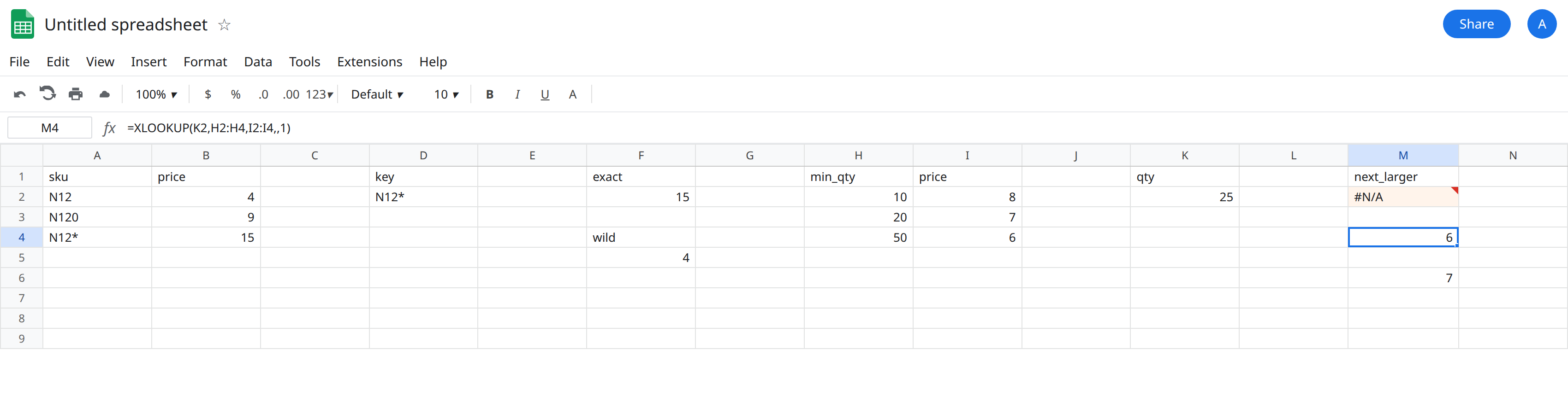
Leave M2 as #N/A. Leave F5 as 4 if the star sku was the one you wanted.

What is actually wrong

• Argument order is search_key, lookup_range, result_range, if_not_found, match_mode, search_mode. A single -1 typed in the fifth slot is next smaller. The same -1 in the sixth slot is last-to-first. XLOOKUP search_mode passes 0 then -1 so the match stays exact. This page passes 2 or 1 or -1 and leaves search mode at the default.
• Mode 0 does not treat * or ? as patterns. F2 finds the literal star. People who learned COUNTIF wildcards expect the star to “just work.” It does not, until mode 2.
• Mode 2 uses * for any run of characters and ? for one character. The first match wins. N12* matches N12, N120, and N12*. F5 returns the first of those, price 4. if_not_found never runs, because a match existed. A label of "missing" would be a lie on this row.
• ~ escapes a wildcard in mode 2. It is unnecessary noise in mode 0, and it is required in mode 2 when the sku really contains a star.
• Mode 1 walks to the next larger value. A quantity break copied from VLOOKUP(..., TRUE) wants the next smaller break (price 7), which is mode -1 (M6), not mode 1 (M4). M4’s 6 is a successful lookup of the wrong band. There is no error triangle.
• These neighbor modes are not binary search. Binary search is search_mode 2 or -2, and it wants a sorted range. Mixing “approx” in your notes with the sixth argument sends you to the other page.

This is not MATCH type 1. See MATCH approx unsorted. MATCH returns a position and defaults to approximate. XLOOKUP defaults to exact.

Fix

Leave F5 and M2 on the sheet so the two wrong shapes stay visible: a wildcard that hit the prefix, and an exact miss of an in-between quantity.

Literal star sku. Keep F2: =XLOOKUP(D2,A2:A4,B2:B4). Or keep the escaped mode 2 in F7 if the rest of that formula must stay in wildcard mode.

A real pattern. Mode 2 without a tilde, and accept the first hit. If several skus match, narrow the pattern or sort the list so the row you want is first. Do not add search_mode -1 and hope it means “the star one.”

Quantity breaks. For “largest minimum still <= qty,” use mode -1: M6 is 7. For “smallest minimum still >= qty,” use mode 1: M4 is 6. Say which one the price list is. Do not leave the fifth argument empty and expect a band. Empty means exact, and M2 is #N/A.

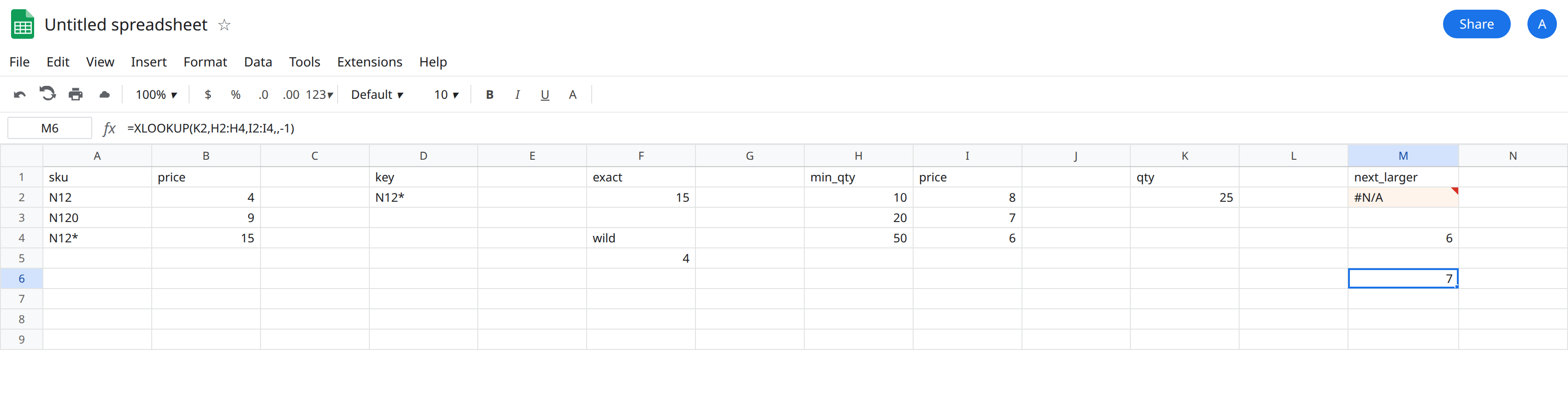
Do not wrap F5 in IFNA. F5 is a number. Do not wrap M4 either. Wrap M2 only when a missing exact key should print a label: =XLOOKUP(K2,H2:H4,I2:I4,"no break"). See IFERROR vs IFNA. IFERROR would also hide a #REF! from a bad column index in a different formula.

If the star changed which row came back, you changed match_mode to 2. If the band price jumped from 7 to 6, you used next larger instead of next smaller. If the formula has -1 in the sixth spot, you are on the search-mode page, not this one.