QUERY headers 0 and 1 decide whether the first row is a label or a data row

QUERY(data, query, [headers]) takes a third argument: how many rows at the top of data are headers. 1 means the first row is labels. Those labels are not filtered by where, and they are not data. 0 means every row is data, including a row that looks like titles. Omit the argument, or pass -1, and Sheets guesses. The guess is how a header becomes a sku, or a sku becomes a header, with no #REF!. On IMPORTRANGE the same number applies, and the columns are Col1, Col2, not A, B.

select A on an import is Col1 vs A. Allow access on the import itself is IMPORTRANGE access. Keep the Google Sheets UI in English. Sheet Error is an independent formula-error library, not a Google product.

Recreate it on a blank sheet

1. Open a blank spreadsheet. In A1 type sku, B1 name. A2 101, B2 Widget. A3 102, B3 Gadget. Row 1 is labels. Rows 2 and 3 are data. You can run every local formula before you involve a second file.

headers 1 on a range that includes the labels. In D1 type h1. In D2 enter =QUERY(A1:B3,"select A",1). The spill’s header is sku. Under it: 101 and 102. Both skus are data. That block is the control.

headers 0 keeps the label row as data. In D6 type h0. In D7 enter =QUERY(A1:B3,"select A",0). There is no header row inside A1:B3 as far as this call is concerned. The generated label is the column id, and the values include the word sku, then 101, then 102. The word sku is a row you can filter. In D11 enter =QUERY(A1:B3,"select A where A = 'sku'",0). D11 returns sku. The same where with headers 1 does not, because sku is not data in D2. Leave D7 as the spill that contains the word sku in the body.

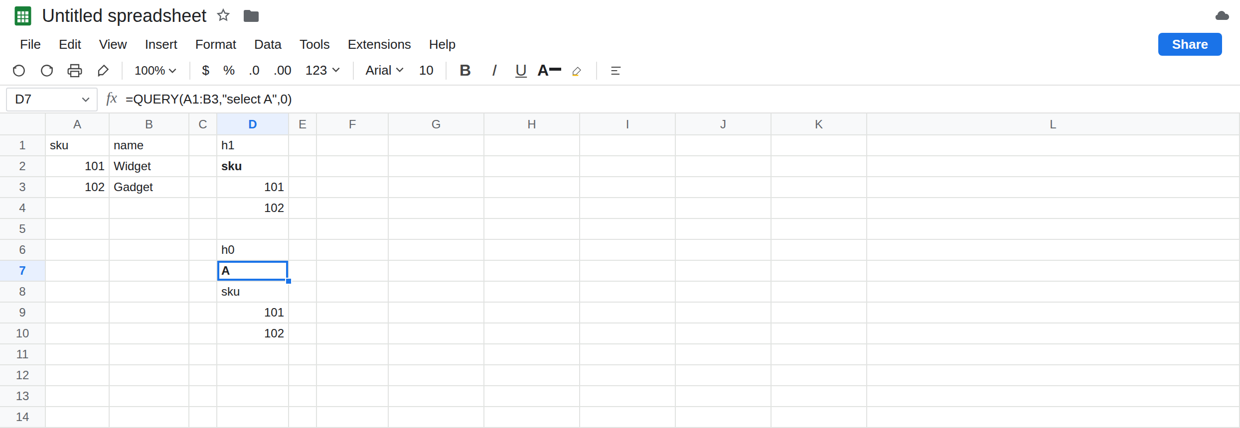
headers 1 on a range that already starts at the data. In F1 type ate. In F2 enter =QUERY(A2:B3,"select A",1). A2:B3 is 101 / Widget and 102 / Gadget. There is no label row in that range. Headers 1 consumes 101 as the label. The only value under it is 102. Widget’s sku is the header text. In F6 enter =QUERY(A2:B3,"select A where A = 101",1). The data rows are only 102. The where does not see 101. F6 is #N/A (query completed with an empty output) or a header-only spill of 101 with no body row. Either way, 101 is not a data hit. Leave F2 as the eaten sku.

The guess. =QUERY(A1:B3,"select A") with no third argument often matches D2, because row 1 is text above numbers. Two numeric rows and no label do not give you that contract. Write 0 or 1.

IMPORTRANGE uses the same switch. When a second spreadsheet’s Sheet1!A1:B3 is the source, the local control is the shape above. On the target:

=QUERY(IMPORTRANGE("SOURCE_ID","Sheet1!A1:B3"),"select Col1",1)

matches D2: label sku, values 101 and 102, and the column is Col1.

=QUERY(IMPORTRANGE("SOURCE_ID","Sheet1!A2:B3"),"select Col1",1)

matches F2: 101 is eaten as the label because the range started at the first data row and you still passed 1. Pass 0 when the import range has no label row. select A on either import is the wrong name; that #N/A is Col1 vs A. If the cell says you need to connect these sheets, stop and use IMPORTRANGE access. Replace SOURCE_ID with the real id. Leave the local F2 broken even if you never open the second file.

Leave F2 with 102 as the only data sku. Leave D2 with both skus.

What is actually wrong

• headers is a count of rows, not a yes/no in the abstract. 1 always means “the first row of this range.” If the range is A1:B, that row should be the titles. If the range is A2:B, that row is the first sku, and 1 hides it from where.
• 0 does the opposite. Titles stay in the data. A where Col1 is not null keeps them. A numeric comparison skips the word sku quietly, so the bug shows up as an extra text row or as a column that QUERY treats as mixed type. Mixed type is QUERY mixed dates when the column was supposed to be dates. Here the extra text is the header you included.
• -1 and omitting the argument are the guess. Text in row 1 and numbers below often guess 1. Two number rows do not give you a contract. Write 0 or 1.
• IMPORTRANGE does not change the third argument. It changes column names to Col1. A format clause on that array is QUERY format, and it will not put 101 back into the body.
• The header row is returned even when where matches nothing. See QUERY no rows after you know 101 was not consumed as a label.

This is not QUERY LIMIT / OFFSET. limit drops rows from the result. headers decides what the input’s first row is.

This is not a locale parse. The formulas use commas because the recreate is a United States argument separator. See locale semicolons if the formula itself is #ERROR!.

Fix

Leave F2 and D7 as the wrong counts.

Range includes titles: pass 1. Keep D2. Both skus stay in the body.

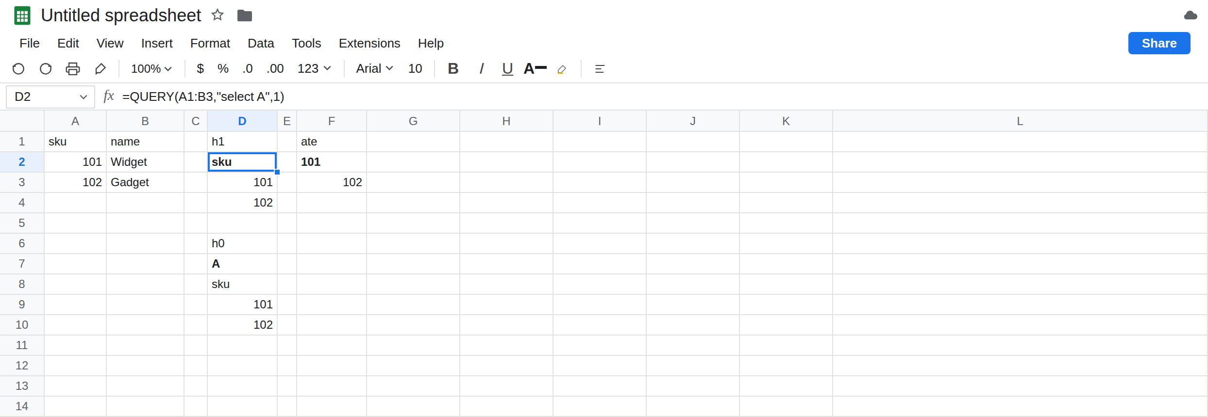
Range starts on the first data row: pass 0. In H2 enter =QUERY(A2:B3,"select A",0). H2’s body is 101 and 102. The label is the generated column id, not 101. On an import that starts at A2, use that 0 and Col1:

=QUERY(IMPORTRANGE("SOURCE_ID","Sheet1!A2:B3"),"select Col1",0)

Prefer one habit. Import A1:B and pass 1, so the source titles stay the labels. Do not mix A2:B with 1.

Do not wrap F6 in IFNA until you know 101 is actually absent. See IFERROR vs IFNA. If 101 is sitting in the header of F2, it is not absent.

If the first sku shows up as the column title, headers is 1 on a range with no title row. If the word sku shows up as a value, headers is 0 on a range that included titles. If select A fails on IMPORTRANGE, switch to Col1 before you touch the header count. If the import is #REF! and asks you to connect, the header number is not the bug yet.

1 vs 0 vs the eaten sku

QUERY(A1:B3,"select A",1) lists 101 and 102 under sku. Headers 0 lists the word sku as data. Headers 1 on A2:B3 labels 101 and lists only 102. The import form is the same count with Col1.