SUBTOTAL 9 includes rows you hid by hand; 109 leaves them out

SUBTOTAL(function_num, range) uses function_num for two choices at once. The units digit is the aggregate: 9 is SUM, 1 is AVERAGE, 2 is COUNT, 3 is COUNTA. Adding 100 does not switch SUM to AVERAGE. It switches whether rows you hid with Hide row are included. 9 sums and includes those rows. 109 sums and excludes them. 1 averages and includes them. 101 averages and excludes them. Filtered-out rows are already excluded for every code. Choosing 109 is not what “turns on” a filter.

The filter-versus-hide walkthrough on the same codes is SUBTOTAL hidden rows. Nested SUBTOTAL results dropped from the total are nested SUBTOTAL. Excel’s AGGREGATE option codes are a different table, and Sheets has no AGGREGATE. See AGGREGATE codes. Keep the Google Sheets UI in English. Sheet Error is an independent formula-error library, not a Google product.

Recreate it on a blank sheet

1. Open a blank spreadsheet. In A1 type qty. A2 5. A3 15. A4 25. A5 35. The plain sum is 80. The average is 20. Four numeric rows.

Nothing hidden. In C1 type sum9. In C2 enter =SUBTOTAL(9,A2:A5). C2 is 80. In D1 type sum109. In D2 enter =SUBTOTAL(109,A2:A5). D2 is 80. In E1 type avg1. In E2 enter =SUBTOTAL(1,A2:A5). E2 is 20. In F1 type avg101. In F2 enter =SUBTOTAL(101,A2:A5). F2 is 20. Four controls. 109 is not a different statistic from 9 while every row is visible.

Hide one row by hand. Right-click the row header for row 4 (the 25) and choose Hide row. C2 stays 80. Code 9 still adds the hidden 25. D2 becomes 55 (5+15+35). Code 109 skips the row you hid. E2 stays 20 (the average of all four numbers, hidden row included). F2 becomes 18.333…, the average of 5, 15, and 35. The 100 you added changed who is in the aggregate. It did not change SUM into AVERAGE. Leave row 4 hidden.

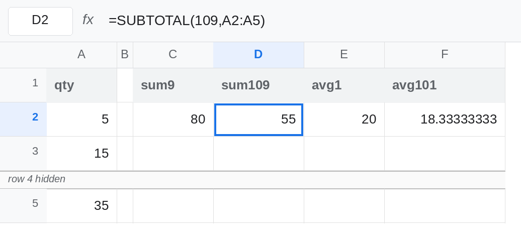
COUNT uses 2 and 102, not 9. In C4 enter =SUBTOTAL(2,A2:A5). C4 is 4. Code 2 is COUNT, and the 1–11 family includes the manually hidden row, so the hidden 25 is still a number being counted. In D4 enter =SUBTOTAL(102,A2:A5). D4 is 3. People who memorize “9 means subtotal” and then write 109 for a count are still summing. =SUBTOTAL(3,A2:A5) is COUNTA, which on this numeric column matches COUNT. The units digit is the function. The hundreds digit is only the hide switch.

A filter does not split 9 from 109. Unhide row 4. Select A1:A5. Data → Create a filter. Clear 35 in the filter menu. Row 5 drops out because of the filter. C2 and D2 both become 45 (5+15+25). The manual-hide switch did nothing, because nobody used Hide row. =SUM(A2:A5) stays 80. Turn the filter off with Data → Remove filter when you are done reading it. The longer filter story is SUBTOTAL hidden rows.

Leave row 4 hidden again if you want C2 at 80 and D2 at 55 while you read the codes.

What is actually wrong

• function_num 9 and 109 are the same aggregate. Both are SUM. The same pairing is 1/101 AVERAGE, 2/102 COUNT, 3/103 COUNTA, 4/104 MAX, 5/105 MIN. The added 100 is “exclude rows hidden with Hide row.”
• A cheat sheet that lists only 1 through 11 is not wrong about the aggregate. It is incomplete about manual hides. A report that still includes a row you collapsed for printing is code 9 (or 1, or 2) doing what that family does.
• Filters are outside this switch. Both families skip filtered rows. If 9 and 109 match while a filter is on, that match is expected. Hide a row by hand to see them diverge.
• SUM and AVERAGE ignore the codes, the filter, and the manual hide. Replacing SUBTOTAL with SUM to “simplify” puts the hidden 25 back into the total.
• Another SUBTOTAL sitting inside the range is ignored by every code. That is nested SUBTOTAL, not the 100 switch. A total that looks short with nothing hidden is often a nested subtotal, not a hidden row.

This is not Excel AGGREGATE, where a second argument chooses errors and hidden rows from a different list. See AGGREGATE codes. In Google Sheets that function is #NAME?.

Fix

Leave the hidden-row contrast in place: C2 is 80, D2 is 55.

Pick the aggregate, then add 100 only if Hide row should drop out. For a printed view that hides detail rows, use 109 for the sum and 101 for the average. For a total that must include rows a colleague hid while leaving a filter honored, use 9 or 1. Write the code you mean next to the label (sum, ignore manual hides) so the next edit does not “correct” 109 back to 9.

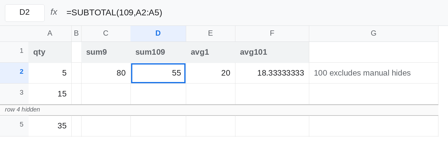
Do not encode the aggregate in the hundreds digit. 101 is not “SUM, but stricter.” It is AVERAGE without manually hidden rows. If D2 was supposed to be a count of visible numbers, the code is 102, and on this sheet that count is 3 while row 4 stays hidden.

If 9 and 109 are equal, no row in the range is manually hidden. Look at the filter, or at a nested SUBTOTAL, before you change the code. If they differ by exactly the cells you hid with Hide row, the codes are working, and the one that matches the report is the one to keep.