Fix FILTER #N/A in Google Sheets (no matches and mismatched range sizes)

FILTER can land as #N/A for two different reasons. One is an empty result. The other is a size error. Both cells show #N/A. They are not the same problem. Read the tooltip before you wrap anything. IFNA is correct for zero rows. It does nothing useful for mismatched heights, and IFERROR will hide both as if they were empty.

Recreate it on a blank sheet

1. Open a blank spreadsheet. Leave the tab named Sheet1. In A1 type sku, B1 name.
2. In A2 type 101. B2 Widget. A3 102. B3 Gadget. A4 103. B4 Lamp.

Recreate 1 — no matches. In D1 type no_match. In D2 enter =FILTER(A2:B4,A2:A4=999). The cell shows #N/A. The tooltip is No matches are found in FILTER evaluation.

D2 selected. Formula bar shows =FILTER(A2,A2=999). D2 is #N/A. Tooltip: No matches are found in FILTER evaluation.

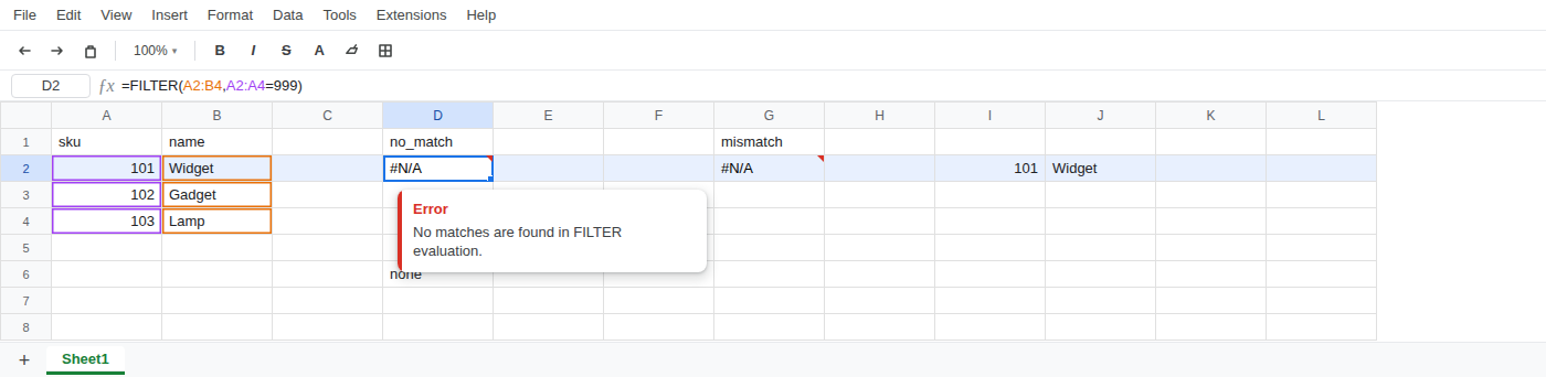
Leave D2 as the broken no-match formula.

Recreate 2 — mismatched range sizes. In G1 type mismatch. In G2 enter =FILTER(A2:B4,A2:A5=101). A2:B4 is three rows. The condition A2:A5 is four rows. The cell shows #N/A. The tooltip is FILTER has mismatched range sizes. Expected row count: 3. column count: 1. Actual row count: 4, column count: 1.

G2 selected. Formula bar shows =FILTER(A2,A2=101). G2 is #N/A. Tooltip: FILTER has mismatched range sizes. Expected row count: 3. column count: 1. Actual row count: 4, column count: 1.

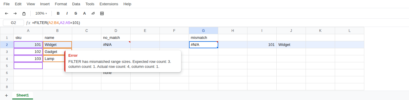
Leave G2 as the broken mismatch formula. That second cell is still #N/A. It is not #REF!. Sku 101 is on the sheet. The size error is not a miss.

What is actually wrong

No matches: FILTER found zero rows. Sku 999 is not in A2:A4. That is a real empty result, still shown as #N/A. The formula ran. The condition is the same height as the data. Sheets has nothing to spill. Confirm by changing 999 to 101. D2 spills 101 / Widget. Put 999 back so the empty result returns.

Mismatch: the range and the condition must be the same height. A2:B4 is three rows. A2:A5 is four. The extra row in A2:A5 is a size error. Still #N/A, not #REF!. Changing 101 to 999 on G2 will not diagnose it. The tooltip already told you the row counts. Make the heights equal first. Then you can talk about zero rows.

COUNTIFS / SUMIFS with ranges of different heights is #VALUE!, not this #N/A. See COUNTIFS range size. Do not copy a COUNTIFS size fix onto FILTER and expect the error value to match.

This is not a VLOOKUP miss for a key you can see (number vs text, a trailing space). See VLOOKUP no match and what #N/A means. FILTER is not searching with a column index.

This is not a VLOOKUP column-index #REF!, a UNIQUE overwrite #REF!, a circular #REF!, or IMPORTRANGE waiting for Allow access. Those are different errors. This page is two FILTER #N/A cases. See VLOOKUP bad index, SORT / UNIQUE spill, circular dependency, and IMPORTRANGE access only if the cell is #REF!.

This is not QUERY year() on mixed dates, and not select A on IMPORTRANGE. See QUERY mixed dates and Col1 vs A.

Fix

Leave D2 as the broken no-match formula. Leave G2 as the broken mismatch formula.

Empty FILTER: wrap with IFNA. In D6 enter =IFNA(FILTER(A2:B4,A2:A4=999),"none"). The cell shows none.

D6 selected. Formula bar shows =IFNA(FILTER(A2,A2=999),"none"). D6 is none. D2 is still #N/A. A working FILTER for 101 spills 101 / Widget.

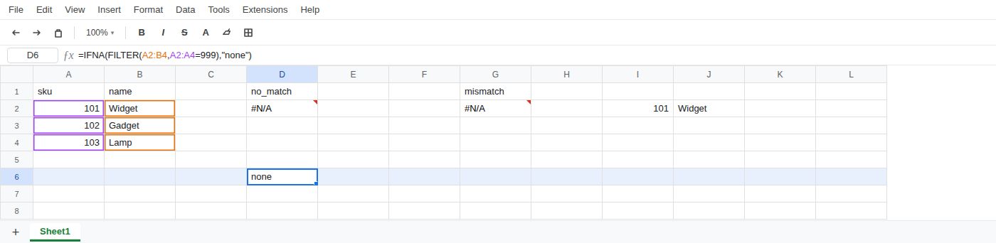
Use IFNA, not IFERROR, for the empty result. IFERROR would also turn G2’s size error into none, and you would never fix the heights. See IFERROR vs IFNA.

Mismatch: same height. Do not wrap G2. Change the condition to A2:A4. A working formula on sku 101: =FILTER(A2:B4,A2:A4=101) spills 101 / Widget. Put that in G6 if you want it next to the broken G2.

Do not change File > Settings locale. Do not wrap this in IMPORTRANGE. Do not switch the condition to QUERY Col1.

If FILTER is #N/A, first ask whether it found zero rows or whether the ranges are different heights. Those two #N/A values are not interchangeable. The tooltip is the split.