GETPIVOTDATA on a month group is #REF! when you pass the original date

GETPIVOTDATA looks up a pivot item by the label the pivot shows, not by a date that merely falls inside that bucket. Group the row field by month and the pivot stops listing 15 Jan 2024 as its own item. It lists a group label, often Jan, under a field name that includes the group, such as opened - Month. A formula that still passes DATE(2024,1,15) and the original column name is #REF!. The January total is on the pivot. The arguments do not name it.

A missing field or a renamed value header, with no date grouping, is GETPIVOTDATA. A pivot that shows yesterday’s numbers is pivot not refreshing. QUERY’s pivot clause is QUERY PIVOT. Keep the Google Sheets UI in English. Locale United States. Sheet Error is an independent formula-error library, not a Google product.

Recreate it on a blank sheet

1. Open a blank spreadsheet. In A1 type opened, B1 qty. In A2 enter =DATE(2024,1,15). B2 10. In A3 enter =DATE(2024,1,20). B3 3. In A4 enter =DATE(2024,2,2). B4 4. Format A2:A4 as dates. January’s qty is 13. February’s is 4.

Build the pivot and group the dates. Select A1:B4. Insert → Pivot table. Put it on the same sheet, starting at D1. In the pivot editor, add Rows: opened. Add Values: qty, summarized by SUM. You should see one row per source date.

Right-click a date in the pivot’s row labels. Choose Create pivot date group → Month. The row labels collapse to month groups. On a United States locale those labels are typically Jan and Feb. The row field in the editor is no longer only opened. It shows a grouped name, typically opened - Month. The January value is 13. If the menu or the label text differs, use the words on your pivot for the rest of this page. Do not translate them.

Let Sheets write a formula that works. Click F1. Type = and click the January total (13). Sheets inserts GETPIVOTDATA. The formula names the value field, the pivot anchor, the grouped field, and the item Jan (or whatever label you clicked). F1 shows 13. That is the control. If Sheets inserted a plain cell reference instead, type GETPIVOTDATA yourself using the value name and the row label you see, including the grouped field name.

The original date is not an item. In F3 enter =GETPIVOTDATA("SUM of qty",D1,"opened",DATE(2024,1,15)). Use the value-field text F1 actually uses if it is not SUM of qty. F3 is #REF!. The tooltip says the field name or the field combination is not in the pivot. 15 Jan 2024 is a source row. After the month group it is not a pivot item, and opened may no longer be the field name the pivot is showing. Leave F3 broken.

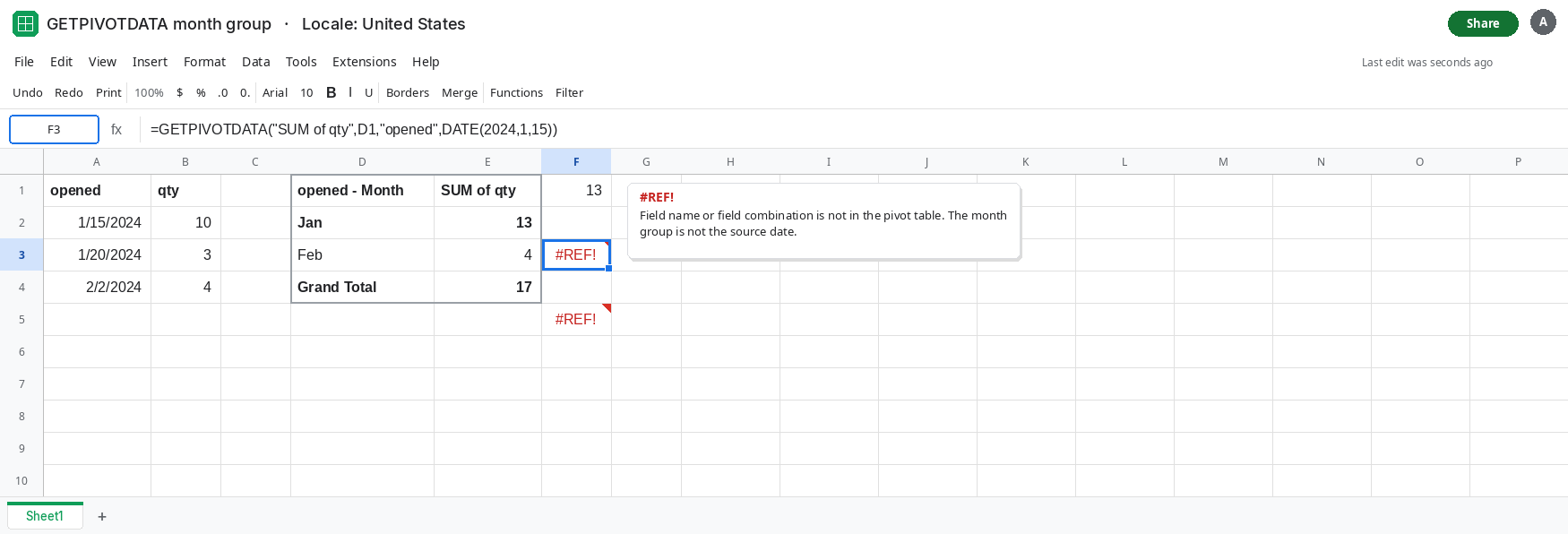
A date that is only formatted like the label still fails if the field name is the raw column. In F5 enter =GETPIVOTDATA("SUM of qty",D1,"opened","Jan"). F5 is #REF! when the pivot’s field is the grouped name rather than opened. The item text is right and the field name is the pre-group column. Leave F5 broken if it is #REF!.

Leave F3 broken. Leave F1 as 13.

What is actually wrong

• Grouping replaces the items. GETPIVOTDATA will not search “which group contains this date.” It compares the argument to the labels on the pivot. DATE(2024,1,15) equals none of those labels.
• The field argument has to be the name in the pivot editor after the group, not the header in row 1 of the source, when those strings differ. A custom header makes this stricter: the function wants the custom name. Google’s own description of GETPIVOTDATA says a custom heading replaces the source column name.
• Clicking the cell is the reliable way to learn both strings. The quotes in F1 are the contract. Editing them back to the source date breaks a formula that was working.
• An ungrouped pivot does accept a source date, and the date has to match the source cell’s value. Grouping is what changes the contract. If you remove the date group, F3’s shape can start working and F1’s Jan item can start failing. See GETPIVOTDATA for a wrong item with no grouping involved.
• #REF! here is not a deleted cell on the grid. The formula is still a function call. See after you delete if the formula bar itself contains #REF! where a cell used to be.

This is not a stale pivot. The January total updates when the source qtys change, and F3 stays #REF! either way. See pivot not refreshing when the pivot number itself is old.

Fix

Leave F3 and F5 broken.

Copy the grouped field name and the group label from the pivot. In H1 enter the formula Sheets wrote in F1, or click the January total again. H1 is 13. The item is the label you see (Jan), and the field is the grouped name you see (opened - Month or the equivalent on your editor).

In H3 enter a February lookup by changing only the item to the February label, for example Feb. H3 is 4 when that label is what the pivot shows. Do not pass DATE(2024,2,2).

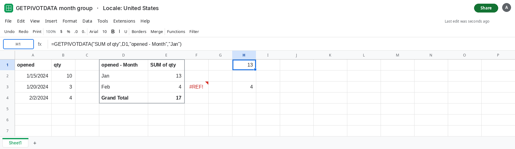
If the label is built from a cell, format that cell to the same text the pivot shows, and pass the text. A date serial in the criterion cell will not equal Jan. TEXT of a date, with a format that produces Jan, is the right type of argument. Check it against the pivot label character for character, including the year if your group label includes a year.

Or skip GETPIVOTDATA for this question. A month total from the source is =SUMIFS(B2:B4,A2:A4,">="&DATE(2024,1,1),A2:A4,"<"&DATE(2024,2,1)), which is 13, and it does not care how the pivot is grouped. Use GETPIVOTDATA when you want the pivot’s number, including its filters. Use SUMIFS when you want the source.

If F3 is #REF! and the pivot rows say Jan rather than 15 Jan 2024, the formula is still asking for the source date. If F1 returns 13 with Jan in the formula bar, that is the item string to copy. If the value field was renamed, match that name too. See GETPIVOTDATA.