SUMIFS puts the sum range first, so a SUMIF-shaped call totals the wrong column

SUMIF(criteria_range, criterion, [sum_range]) puts the test first. SUMIFS(sum_range, criteria_range1, criterion1, …) puts the numbers you add first. The extra S is not the only change. A formula copied from a SUMIF habit, =SUMIFS(B2:B4,A2:A4,">1") when you meant to add column A and test column B, adds the wrong field. Both columns are numbers, so the result is a normal total. There is no triangle. The other habit, dropping the criterion into the second argument the way SUMIF does, is =SUMIFS(A2:A4,">10",B2:B4). The second argument is not a range of the same height. That one is #VALUE!.

Sheet Error is an independent formula-error library, not a Google product. A criteria range that is taller than the sum range is COUNTIFS range size. Dates that look equal and do not match are SUMIFS date text. Wildcards in the criterion are SUMIFS wildcards. Keep the Google Sheets UI in English.

Recreate it on a blank sheet

1. Open a blank spreadsheet. In A1 type qty, B1 price. A2 2, B2 10. A3 5, B3 4. A4 1, B4 20. Quantities are 2, 5, and 1. Prices are 10, 4, and 20.

SUMIF, criteria first, the shape people memorize. In D1 type sumif. In D2 enter =SUMIF(B2:B4,">10",A2:A4). The test is the price. The sum is the quantity. Only the price 20 is greater than 10. D2 is 1. That cell is the control for the question “how many units sold above a price of 10.”

SUMIFS with the sum range first, same question. In D4 enter =SUMIFS(A2:A4,B2:B4,">10"). D4 is 1. Same total. The arguments are not in the SUMIF order. The sum range is first. This is the working SUMIFS. Leave D4 as 1.

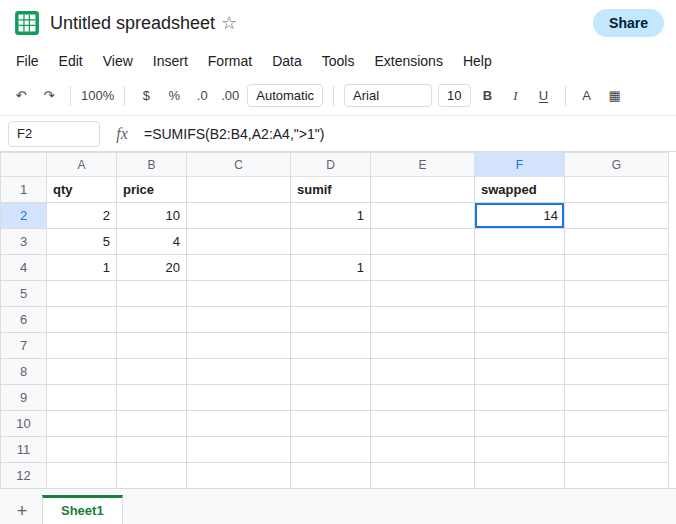
The swapped numeric call. In F1 type swapped. In F2 enter =SUMIFS(B2:B4,A2:A4,">1"). This adds prices where the quantity is greater than 1. Quantities 2 and 5 qualify. Prices 10 and 4. F2 is 14. No error. If the question was still “units with price above 10,” 14 is a price total. It looks like a plausible revenue number. Leave F2 as 14.

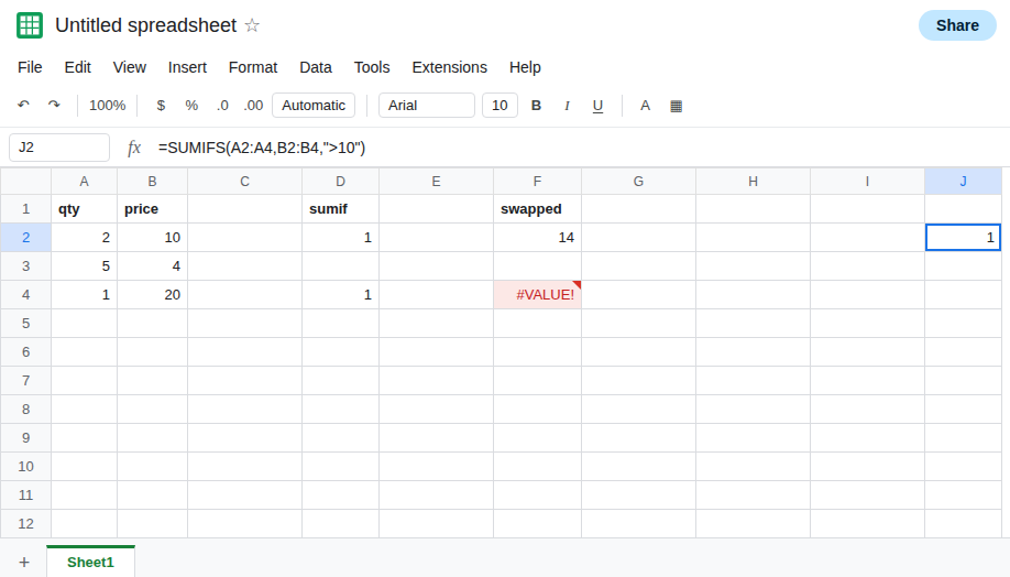
The SUMIF argument order inside SUMIFS. In F4 enter =SUMIFS(A2:A4,">10",B2:B4). The second argument is the text ">10", where a criteria range should be. The third argument is a range, where a criterion should be. F4 is #VALUE!. The tooltip is about the arrays being different sizes, or about the criteria range. Read it. Leave F4 broken. Do not “fix” F2 by copying F4. F2 is a successful sum of the wrong column. F4 never summed.

A text criteria column makes the swap obvious. In H2 enter =SUMIFS(A2:A4,A2:A4,">10") only as a contrast if you replace column A with regions. Skip that if you want to keep the numeric trap. The dangerous case is F2, where both ranges are numbers and 14 does not announce itself.

What is actually wrong

• SUMIFS requires the sum range in position one. Every later argument is a pair: a range to test, then the test. SUMIF allows the sum range to be omitted or placed third. Muscle memory from SUMIF fills SUMIFS backwards.
• Two numeric ranges of the same height are legal in either order. The function adds whichever range is first, on the rows where the later test passes. F2 is 14 because prices were first. The criteria ">1" was applied to quantities. Nothing in the cell says “you swapped these.”
• A criterion in the range slot is a size error. One text value is not three rows. F4 is #VALUE!. That tooltip is COUNTIFS range size when the ranges really differ in height. Here the height differs because a criterion was asked to be a range. Same token, a different edit.
• Same-size ranges that start on different rows do not #VALUE!. They pair by position and can total the wrong rows, including 0. Check the start row after the order is right.
• Text in the sum range is skipped, so a swap that puts regions first totals 0 with no triangle. See SUMIF text numbers. F2 is worse than that zero, because 14 looks real.

Fix

Leave F2 as 14 and F4 as #VALUE!. Leave D4 as 1.

Put the column you add in the first argument. In J2 enter =SUMIFS(A2:A4,B2:B4,">10"). J2 is 1, the units whose price is above 10. The criteria range is B, the prices. The criterion stays a string in the third argument, not in the second.

When you only have one test, SUMIF’s order is still legal. D2 is that formula. Use it if you do not need a second criterion. The moment you add another test, you need SUMIFS, and the sum range moves to the front. Do not keep the SUMIF order and insert the new test in the middle.

A second test is another pair at the end. =SUMIFS(A2:A4,B2:B4,">10",A2:A4,">0") still adds quantities. Both criteria ranges are the same height as A2:A4. The sum range stays first.

Do not wrap F2 in IFERROR. There is no error to catch. The total is the other column. See IFERROR hides cause.

If SUMIFS returns a calm number and the first range is not the column you meant to add, the argument order is the bug. If the cell is #VALUE! and the second argument is a criterion rather than a range, move that criterion to the third argument and put a range second. If the tooltip says the arrays differ in size and every argument is already a range, you are on the size page.